I describe a simple method for constructing a sequence of points, that is based on a low discrepancy quasirandom sequence but exhibits enhanced isotropic blue noise properties. This results in fast convergence rates with minimal aliasing artifacts.
First published: 13th November, 2018
Last updated: 2nd March, 2020
Introduction
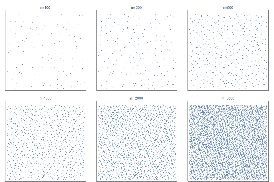
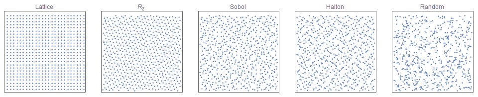
Quasirandom low discrepancy sequences are useful to create distributions that appear less regular then lattices, but more regular than simple random distributions (see figure 2). They play a large role in many numerical computing applications, including physics, finance and in more recent decades computer graphics.
The classic paper on how using quasirandom sampling over uniform sampling can improve 2D images is “Stochastic Sampling in Computer Graphics” [Cook, 1986]. In more recent decades, quasirandom sampling has become a major tool in 3D rendering. Rendering (and samplers) can utilize either the CPU or GPU for calculations. For an excellent primer on their use in 3D rendering, see “Anti-aliased Low Discrepancy Samplers for Monte Carlo Estimators in Physically Based Rendering” [Perrier, 2108]. In this paper, she describes the task of 3D rendering (see figure 3) as follows:
“When displaying a 3-D object on a computer screen, this 3-D scene is turned into a 2-D image, which is a set of organized colored pixels. We call Rendering the process that aims at finding the correct color to give those pixels. This is done by simulating and integrating all the light,….we numerically approximate the equation by taking random samples in the integration domain and approximating the integrand value using Monte Carlo methods….A stochastic sampler should minimize the variance in integration to converge to a correct approximation using as few samples as possible. Many different samplers exist that we roughly regroup into two families:
– Blue Noise samplers, that have a low integration variance while generating unstructured point sets. The issue with those samplers is that they are often slow to generate a point set
– Low Discrepancy samplers, that minimize the variance in integration and are able to generate and enrich a point set very quickly. However, they present a lot of structural artifacts when used in Rendering.”
In recent years, efforts have been made to combine to the anti-aliasing advantages of jittered sampling, with the fast convergence rates (low variance) associated with low discrepancy quasirandom sequences [Christensen, 2018]. With this same goal, I present a new and different method to construct an infinite point sequence, that is extremely simple, fast to calculate, progressive, fully deterministic, exhibits fast convergence rates (low variance), with desirable isotropic, blue noise spectra and therefore results in minimal artifacts.
So here goes…
 | 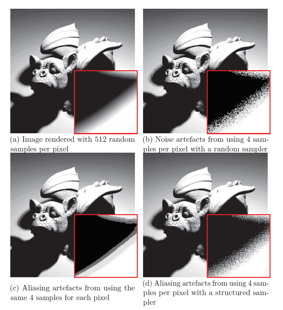 |
| Figure 3. Rendering in 3D (left). Undesirable aliasing artifacts often arise in sampling processes (right). Source:[Perrier, 2018] | |
Outline
- simple jittered (finite) point sets
- jittered quasirandom point sets
- jittering of (infinite) quasirandom sequences
- QMC convergence comparisons
- summary
- example code
Simple Jittered Sampling
The most basic jittered (perturbed) point sets are the jittered grids. In this case, the sample space is subdivided into a grid of $m \times m$ square regions. Instead of merely selecting a point at the center of each cell, any (pseudo-) random point within each cell is selected.The advantages of jittered grid sampling is that it is trivial to understand, simple to implement, and extremely fast to compute. It has the obvious limitation that $N$ must be a perfect square.
Although rectangular stratified sampling can ease this limitation by simply requiring $N$ to be the product of two appropriate integers, I describe a different approach that is is informative, very elegant but less well known. Without loss of generality, assume that our sample space is the unit square $[0,1)^2$.
We define the Fibonacci lattice as of $N$ points where:
$$ \pmb{p}_i(x,y) = \left( \frac{i-0.5}{N}, \left\{ \frac{i}{\phi} \right\}\; \right); \quad \textrm{for } \; i=1,2,3,…, N. \tag{1}$$
where $\phi \simeq 1.618033988$ is the golden ratio, and $\{ x \} $ denotes the fractional part of $x$. Note that in computing, this fractional operator is usually written and implemented as $ x \; \%1$ (pronounced ‘mod 1’), and as this post as mainly geared towards computing applications we shall use this notation from here onwards.
Note that the Fibonacci lattice is a very elegant method to place any number of points in the unit square in an extremely regular manner. For example, figure 2a shows the standard Fibonacci lattice for N=41 points. For jittered sampling, instead of selecting the center of each disk for our sample points, we can simply select a point $\tilde{p_i}$, inside each of the $N$ disks (see figure 4b).
$$ \tilde{\pmb{p}_i}(x,y) = \pmb{p}_i(x,y) + \pmb{\epsilon}_i (\delta_0/ \sqrt{N}),\quad \textrm{where } \delta \simeq 0.78 \tag{2}$$
where $\epsilon_i(r)$ denotes that for the $i$-th term, a random sample is drawn from a circle centered at zero with radius $r$.
Note that a simple direct method to draw a sample uniformly from a circle of radius $r$ is to first draw two uniform random samples $u_1$ and $u_2$, each from the interval $[0,1)$ and then apply the following mapping:
$$ \pmb{\epsilon}_i(r) = \left( r \sqrt{u_1} \cos(2\pi u_2), r \sqrt{u_1} \sin(2 \pi u_2) \right) \tag{3}$$
Of course, you can reduce the degree of jitter simply by selecting a smaller value of $\delta$.

The point distributions, approximate radial power spectra and the fourier spectra of these point sets is shown below.

If you do know $N$ in advance, then this is a simple but effective way to produce an isotropic point set.
Interestingly, although intuitively there is a consistent distance between neighbouring points, the fourier spectrum of the jittered Fibonacci point set does not show the classic blue noise spectrum. Nonetheless this jittered version is very good for many applications and contexts!
However, there are known to be many excellent ways to produce isotropic point sets if $N$ is known in advance. This post mainly explores the lesser studied area of direct constructions for open/infinite isotropic blue noise point sequences, where $N$ is not known in advance.
Furthermore, although the jittered grid and jittered Fibonacci lattice are extremely fast to compute, they also both suffer the disadvantage that the ordering of the points is ‘line-by-line’. Sampling methods where consecutive points are not proximal, but rather are more ‘evenly spread’ out across of the entire sample space, are often preferred. This property is often termed ‘progressive sampling’.
Thus, we explore the viability of constructing progressive isotropic blue noise point sets and sequences.
Jittering quasirandom point sets
A low discrepancy sequence quasirandom sequence is an (infinite) sequence points whose distribution is more evenly spaced than a simple random distribution but less regular than lattices. These sequences are useful in many applications, such as Monte Carlo integration. There are many types of quasirandom sequences, including Weyl/Kronecker, van der Corput / Halton, Niederreiter and Sobol. I discussed these, including a new one in extensive detail in my previous post: “The unreasonable effectiveness of quasirandom sequences“. This post focuses on just one of these – the $R_2$ sequence. For comparative purposes, the Halton sequence and the Sobol’ sequence are also discussed in this post, as these are the most common in current QMC usage.
A brief summary of each of the low discrepancy quasirandom sequences discussed in this post, is as follows.
$\pmb{R_2}$: The $R_2$ sequence is a Kronecker/Weyl/Richtmyer recurrence sequence, introduced in my previous post. It is based on a generalization of the golden ratio, and so can be considered a natural way to construct a generalized Fibonacci lattice that wraps both left-to-right as well as top-to-bottom. It is defined as:
$$ \pmb{t}_n = n \pmb{\alpha} \; \% 1, \quad n=1,2,3,… \tag{4}$$
$$ \textrm{where} \quad \pmb{\alpha} =\left( \frac{1}{\varphi}, \frac{1}{\varphi^2} \right) \;\; \textrm{and} \; \varphi\ \textrm{is the unique positive root of } x^3=x+1. $$
Note that $ \varphi = 1.324717957244746 \ldots$, often called the plastic constant, has many beautiful properties (see also here).
Halton Sequence: the $d$-dimensional Halton sequence is simply $d$ independent Van der Coruput reverse-radix sequences concatenated in a component-wise manner. This post keeps to the common convention of selecting the first $d$ primes numbers for the bases. Thus, in this post, I always use the {2,3}-Halton sequence.
Sobol Sequence: The Sobol’ sequence is known to have many excellent low discrepancy properties, including fast convergence rates. This post constructs the Sobol sequence (along with parameter selection) via Mathematica version 10. The Mathematica documentation states that the Sobol implementation is “closed, proprietary and fully optimized generators provided in Intel’s MKL library“.
Unlike finite point sets, point sequences are infinite. A key advantage of infinite sequences, is that if the error after $N$ terms is still too large, one can simply sample additional points without having to recalculate all prior points. And an advantage of sampling based on quasirandom sequences is that they are progressive. That is, each successive point is proximally distant from the previous one, and the points fill the sample space evenly as the number of sample points increases.
Figure 5 shows these three prototypical low discrepancy sequences, along with their fourier transforms and radial power spectra. We can see that:
- the $R_2$ points are very evenly spaced out. For many applications, this distribution is ideal, but for other applications it is ‘too even’
- clear patterns are visible in all the low discrepancy sequences, which often results in undesirable artifacts appearing in the QMC rendered images.
- the fourier spectra for all the low discrepancy sequences consists of set of spatially regular peaks
- none of the quasirandom point sets are isotropic
- the radial power spectrum for the $R_2$ sequence consists only of a discrete number of peaks.
- the radial power spectra for the Halton and Sobol sequences are continuous but not smooth.
That is, rendering artifacts are a direct result of (i) discrete bright peaks in the fourier spectra, and/or (ii) discrete peaks in the radial power spectrum.
A quick note on the term ‘blue noise’ may be useful here…
In a loose sense, the $R_2$ distribution could be called blue noise because its low (blue) frequencies are clearly suppressed. However, it only consists of discrete peaks, and so may be better termed ‘discrete blue noise’ (or not called blue noise at all). In its more common context, ‘blue noise’ requires (i) an isotropic fourier spectra and (ii) a radial power spectrum that is flat like white noise, but with the low frequencies completely suppressed. For an excellent review of different blue noise spectra see [Heck, 2012]
Further, some authors [Perrier, 2018] note that most implementations of Poisson Disc sampling methods, such as Mitchell’s best candidate, are not strictly blue noise as their power spectra is small but not strictly zero at the lowest frequencies. In this sense, may be better termed ‘approximate blue noise’. They further comment that the difference between almost zero and exactly zero, can have a significantly detrimental effect on convergence rates.)

We would like to combine the anti-aliasing advantages of jittered sampling with the fast convergence rates associated with low discrepancy quasirandom sequences, and thus:
the main aim of this post is simple: to determine the minimum level of jitter to apply to the quasirandom points, such that the all fourier peaks are suppressed, the transform becomes isotropic, and the radial power spectrum for high frequencies becomes flat and even – ideally whilst keeping the lower frequencies suppressed.
Intuitively this critical level of jitter would be closely related to the typical distance (divided by $1/\sqrt{N}$) between neighboring points. Figures 6a shows that the minimum separation between neighboring points for the $R_2$, Halton and Sobol sequences. Note that $R_2$ sequence is the only low discrepancy sequence where the minimum separation between neighboring points falls as slowly as $1/\sqrt{N}$. For Halton and Sobol the separation falls at much faster rate — closer to $1/N$. Similarly, figure 6b shows that the mean separation in $R_2$ between neighboring points is at least $\simeq \delta_0/ \sqrt{N}$ for $\delta_0 /\simeq 0.76 $, all values of $N$. These figures suggest that jittering $R_2$ within a radius of half this value would be ideal. Empirical tests verify this.

Using this approach, the empirically determined critical radius for the jitter for $R_2$, Halton and Sobol equation are given in the following table. Their corresponding point distributions are shown in figure 5. Note that the jitter for Sobol’ sequence has to fall much slower than $\sim 1/\sqrt{N}$ in order to mask the very distinct artifacts and so I don’t recommend it for any application, but is still included here for completeness.
$$ \tilde{\pmb{p}_i}(x,y) = \pmb{p}_i(x,y) + \pmb{\epsilon}_i (k/ \sqrt{N}), \tag{5}$$
\begin{array}{|lr|} \hline
\mathbf{Sequence} & \mathbf{Radius} & \\ \hline
\text{R2} & 0.5 \delta_0 N^{-0.5} & \delta_0 \simeq0.76 \\ \hline
\text{Halton} & 0.5 \delta_0 N^{-0.5} & \delta_0 \simeq 0.45 \\ \hline
\text{Sobol} & 0.5 \delta_0 N^{-0.2} & \delta_0 \simeq 0.08 \\ \hline
\end{array}
Figure 7 shows that jittered R2, jittered Halton and even jittered Sobol produce isotropic, blue noise point distributions.

Figure 7. Jittered points sets (n=2000) based on various quasirandom sequences: (i) $R_2$ , (ii) Halton; and (iii) Sobol, with (iv) random for comparison. Note that the fourier transform of all the quasirandom versions are now isotropic with small but observable blue noise signatures. Also note that the jitter for the Sobol sequence has to be much larger to mask the very large artifacts. Note that the radial power spectra of jittered R2 and jittered Halton appear similar to Owen’s scrambled and jittered grids (not shown), but their fourier spectra are all very different.
It is worth remarking that for the $R_2$, we could alternatively define the critical level of jitter as the ‘maximum level of jitter possible that still ensures that the radial power spectrum is zero for the lowest frequencies‘. Empirically, this definition results in a similar value of $\delta_0 \simeq 0.76$ for $R_2$, but the corresponding levels for Halton and Sobol, would be very much lower than listed above, and need to fall by $1/n$ and not $1/\sqrt{n}$ like it is for $R_2$.
Related to the desirable fourier spectra, constructing point sets with good separation between neighboring points is often highly desirable. The min and mean separation for n=500 points, for various methods is given as follows. The data prefixed with an asterisk are taken directly from the paper, “Progressive Multi-jittered Sample Sequences” [Christensen, 2018] and the ones in boldface are new results. (The standard Halton and Sobol, and random data are common). Data is shown in descending order of mean separation.
\begin{array}{|lr|} \hline
\text{Type} & \text{Mean} & \text{Min}\\ \hline
\mathbf{R2} & 0.0389 & 0.0303 \\ \hline
\text{*best candidate} & 0.0380 & 0.0289 \\ \hline
\text{*pjbn} & 0.0354 & 0.0217 \\ \hline
\text{*pmjbn} & 0.0336 & 0.0105 \\ \hline
\mathbf{jittered R2} & 0.0312 & 0.0118 \\ \hline
\text{*pmj02bn} & 0.0296 & 0.0077 \\ \hline
\text{*pmj02} & 0.0290 & 0.0067 \\ \hline
\text{*pj} & 0.0287 & 0.0055 \\ \hline
\text{*pmj} & 0.0287 & 0.0055 \\ \hline
\text{*Sobol’} & 0.0283 & 0.0055 \\ \hline
\mathbf{*Halton} & 0.0278 & 0.0111 \\ \hline
\mathbf{jittered Sobol} & 0.0277 & 0.0042 \\ \hline
\mathbf{jittered Halton} & 0.0257 & 0.0052 \\ \hline
\mathbf{*Random} & 0.0224 & 0.0014 \\ \hline
\end{array}
It is worthwhile remembering that discrepancy is a formally an area-based measure. It measures the deviation between the point count density of an arbitrary (rectangular) region of the point distribution to the density if the points were distributed in a uniform lattice. In general, low discrepancy sequences are typically associated with good convergence rates.
In contrast to discrepancy, point separation metrics are length-based measures. Intuitively distributions with good point separation are typically low discrepancy, and vice-versa. For this reason, in practice these concepts are very similar and so are often (loosely and incorrectly) used interchangeably. However, there are times when the subtle differences between these various concepts may appear. An optimal low discrepancy point sequence may have a good but not optimal point separation. And similarly, those with ideal point separations may have a good but not optimal discrepancy. Said another way, “best-candidate disc samples have nice spacing between points but uneven distribution overall” [Christensen, 2018]. This may help in gaining a better intuition as to why the Sobol sequence which has excellent convergence rates but only fair point separation; and why approximate disc sampling may have near optimal blue noise characteristics but only fair convergence rates.
Also note that on the min/mean point separation metrics alone, it would seem that the jittered Halton sequences is effectively useless and indiscernible from random noise. However, figure 4 clearly shows that jittered Halton sequence shows less clumps and gaps than random noise. Thus, each sequence has its advantages and disadvantages, and individual metrics usually only give indication to a narrow aspect of its overall characteristics. (Another key metric not indicated in this table is the time it takes to calculate these points sets. Most of the classic blue noise distributions are based on an acceptance/rejection method or annealing-like methods, and so are quite slow compared to those methods that calculate the points directly.)
Thus, as we have all experienced, theoretical metrics often assist in understanding certain aspects, but they should not govern final choices — such choices should rather be determined by whatever real-world measures and constraints are relevant to our particular context.
Jittering infinite point sequences
The coefficient of $1/\sqrt{N}$ in equation (3) means that this expression can only be used for finite point sets.
In many cases, $N$ is not known in advance.
In situations where an approximate range of $N$ is known (eg, $100 < N <1000$) surprisingly good results can be achieved by setting the jitter size to a fixed value $N_{\textrm{avg}}$ within this range. In this example, a value of $N_{\textrm{avg}} \simeq 400$ works well.
However, this approximate method is not entirely satisfying for the purists among us! If we are to properly jitter an infinite sequence, we need to eliminate this dependency on $N$ entirely. Thankfully, it turns out there is a simple substitution which allows us to jitter an infinite sequence with consistently good results. The requisite substitution is:
$$ \frac{1}{\sqrt{N}} \mapsto\frac{1}{2\sqrt{i-i_0}}; \quad \textrm{where } i_0 = 0.700 $$
That is, the size of the jitter for the $i$-the point, is now a strictly decreasing function of $i$.
Thus, the equation for jittering an infinite $R_2$ sequence is now simply: ,
$$ \tilde{\pmb{p}_i} (x,y) \rightarrow \pmb{p}_i(x,y) + \epsilon \left( \frac{k}{2 \sqrt{i-i_0}}\right ) ; \quad \textrm{for } i = 1,2,3,…,N; \quad k \simeq 0.38, \; i_0 = 0.700 \tag{6}$$
The radius of jitter for each of the infinite quasirandom sequences is as follows:
\begin{array}{|lr|} \hline
\mathbf{Sequence} & \mathbf{Radius} & \\ \hline
\text{R}_2 & 0.25 \delta (i – i_0)^{-0.5} & \delta _0\simeq 0.76, & i_0 =0.700 \\ \hline
\text{Halton} & 0.25 \delta (i – i_0)^{-0.5} & \delta_0 \simeq 0.90, & i_0 = 0.700 \\ \hline
\text{Sobol} & 0.4 \delta (i – i_0)^{-0.2} & \delta_0 \simeq 0.16, & i_0 =0.58 \\ \hline
\end{array}
The point distribution of this jittered infinite sequence is shown in figure 1 at the top of this page. Furthermore, as can be seen in figure 8 shows that this adaption from jittering a point set to jittering an infinite sequence has virtually no visible effect on quality!

Calculating jitter
Jitter Shape
So far I have only discussed radial jitter. Empirical tests show that the visual difference is in quality is almost not discernible if the jittering is simply based on a square of side length $\sqrt{\pi}r$ instead of a circle or radius $r$. Although it has a minor negative effect on fourier spectra and some point separation metrics, I have found no measurable difference in convergence rates. Therefore, either for simplicity and/or high-speed computing reasons, the jittering might be simplified to
$$ \pmb{\epsilon}_i(L) = \sqrt{\pi}L (u_1,u_2); \quad (u_1,u_2) \sim U[0,1)^2 \tag{7}$$
Jitter Size
Unlike scrambling or shuffling, which are essentially “all-or-nothing” processes, we can control the amount of jitter that is applied. Thus, we can introduce an adjustable parameter $\lambda$ that specifies the degree of jitter. That is, the jittered points can be simply calculated as:
$$ \tilde{\pmb{p}_i} (x,y) \rightarrow \pmb{p}_i(x,y) + \lambda \frac{\delta}{2\sqrt{N}} \epsilon_i(x,y) ; \quad \textrm{for } i = 1,2,3,…,N; \quad \delta_0 \simeq 0.76, \; \lambda >0\; \tag{8}$$
Figure 9 shows the $R_2$ sequence for N= 600, jittered to varying levels. Note that $\lambda = 0$ corresponds to the original point set without any jittering; for $\lambda = 1$ you have a critical level of jitter; and for $\lambda >2$ you essentially have white noise. For applications that require the pseudo-random placement of items, that are “not too even and not too random”, it seems that for values $\lambda \simeq 50\%$ produce pleasing visual results.

Non-stochastic jitter
This is the final piece of the picture. It should be no surprise that the random functions used in the jitter do not have to be of cryptographic quality. The jitter sampling only has to satisfy some fairly weak criteria, as it only plays a secondary role to the structure of the point distribution. Therefore, where simplicity and/or high speed computing is required, one can (and should?) simply replace all randomization with your favorite high-speed hash functions that output a value in the range $[0,1)$.
However, those purist readers that come from a maths or science background may not find this approach completely satisfying and are no doubt wondering if all the randomization could be replaced with a fully deterministic function.
Thankfully, the answer is a resounding yes!
As far as I know, there are no published methods on how to explicitly and deterministically create isotropic blue noise point sequences. All methods that I know (for finite point sets or open sequences either require shuffling, scrambling, acceptance/rejection methods and/or iterative relaxation -like processes.)
Therefore, one of the main theoretical contributions of this post is to describe how to directly construct a deterministic point sequence with isotropic blue noise.
Not only is it possible that the random jitter be replaced with a fully deterministic function, but the structure of the proposed formula is incredibly similar to the structure for the $R_2$ sequence itself. (And before anyone asks,… as much as I would love to use a low discrepancy sequence for jitter, all empirical tests so far show that the jitter needs to be far ‘less regular’, as each jitter point needs to be a more independent to the previous point than occurs in quasirandom sequences.)
It is generally known that Weyl showed that for any irrational number $\alpha$, the fractional part of multiples of $x$ is uniformly distributed. This obviously forms the basis of the $R_2$ sequence. What is less well known is that he also showed that for almost any number $\beta>1$ , the fractional part of the powers of $\beta$ are uniformly distributed (see fractional part of powers.) and here and here
That is, instead of selecting a random number from the interval $[0,1)$, we can take select a constant $\beta>1$, and then use the $i^{\textrm{th}}$ term of this sequence. Specifically in our case, instead of $u_1$ and $u_2$ being random variates from the interval $[0,1)$, we define $\pmb{u} = (u_1,u_2)$ as follows:
$$ \pmb{u_i} = (\beta_1^i \; \% 1, \beta_2^i \; \%1) \quad \textrm{where } (\beta_1,\beta_2) = \left( \frac{3}{2}, \frac{4}{3} \right). \tag{9} $$
Unless you are using software that automatically handles arbitrary integer lengths (eg Mathematica) you will invariably encounter overflow/underflow issues for $n>70$ if you calculate it directly via the expression
frac = np.pow(1.5,n) %1Therefore, although in theory, $\beta_1,\beta_2$ can be almost any real numbers greater than 1, I chose 3/2 and 4/3 because:
- they give good empirical results, and
- they are of the form $1+1/b$ for integer $b$, whose powers turn out to be easy to calculate.
Some basic code (which can be sped up considerably if interim results are cached) that achieves this is listed in the following section.
QMC integration tests
The most common convergence tests used for QMC comparison is the gaussian curve (figure 7a). As it is a smooth isotropic function, the random sampler converges at $(\mathcal{O}(1/n^{0.5})$ and all the low discrepancy quasirandom sequences generally converge somewhere between $\mathcal{O}(1/n^{0.75}$ and $\mathcal{O}(1/n)$, with the Sobol and $R_2$ sequences converging a bit better than the jittered $R_2$ which in turn is a bit better than Halton.
QMC involving functions with discrete discontinuities is not very common in finance or physics, but is very common in rendering because objects often have sharp boundaries. Therefore, convergent tests involving discontinuous functions illustrate how well the sampling will render edges. That is, how severe the aliasing artifacts will be! We see that compared to the Gaussian, the Sobol sampler for the triangle and disk, shows a notable deterioration in convergence rates. What is most evident, is the poor convergence rate of jittered $R_2$ in the discrete one-dimensional step function. This is, an unfortunate limitation of jittered $R_2$.
Note that these empirical tests, were directly inspired by two excellent papers, “Correlated Multi-jittered Sampling” [Kensler, 2013], and “Progressive multi-jittered Sampling” [Christensen, 2018].

Summary
Combining the results of the previous sections, (eqns 4, 5, 7, 8), formula for the parameterized rectangular jittered $R_2$ finite point set
\begin{align}
\textrm{For } i&=1,2,3,…,N\tag{10} \\
\textrm{define } \tilde{\mathbf{p_i}} &= (\alpha_1 i, \alpha_2 i ) + \frac{\lambda \delta_0 \sqrt{\pi}}{2\sqrt{N}} \left(\beta_1^i, \beta_2^i \right) \;\; \%1 \nonumber \\
& \nonumber \\
\textrm{where } \varphi &= \sqrt[3]{\frac{1}{2} + \frac{\sqrt{69}}{18} } + \sqrt[3]{\frac{1}{2} – \frac{\sqrt{69}}{18} } \simeq 1.324717957244746, \nonumber \\
\alpha &= \left( \frac{1}{\varphi},\frac{1}{\varphi^2} \right) , \; \beta = \left( \frac{3}{2}, \frac{4}{3} \right), \nonumber \\
\delta_0 &\simeq 0.76, \; \lambda >0. \nonumber \\
\end{align}
And similarly, combining the results of the previous sections (eqns 4, 6, 7, 8) , the formula for the parameterized rectangular jittered $R_2$ infinite point sequence can be elegantly expressed as follows:
\begin{align}
\textrm{For } i&=1,2,3,…\tag{11} \\
\textrm{define } \tilde{\mathbf{p_i}} &= (\alpha_1 i, \alpha_2 i ) + \frac{\lambda \delta_0 \sqrt{\pi}}{4\sqrt{i-i_0}} \left(\beta_1^i, \beta_2^i \right) \;\; \%1 & \nonumber \\
\textrm{where } \varphi &= \sqrt[3]{\frac{1}{2} + \frac{\sqrt{69}}{18} } + \sqrt[3]{\frac{1}{2} – \frac{\sqrt{69}}{18} } \simeq 1.324717957244746, \nonumber \\
\alpha &= \left( \frac{1}{\varphi},\frac{1}{\varphi^2} \right) , \; \beta = \left( \frac{3}{2}, \frac{4}{3} \right), \nonumber \\
\textrm{and } \delta_0 &\simeq 0.76, \; i_0 = 0.700, \lambda >0. \nonumber \\
\end{align}
A simple GLSL implementation of this can be found here [Vassvik, 2018].
That is, this method of constructing a two-dimensional point distribution:
- is so simple that it can be expressed in less than 50 lines of basic code;
- is based on a low discrepancy sequence ($R_2$)
- can be either fully deterministic or stochastic depending on your requirements. ($\epsilon$)
- can a finite point set or an infinite point sequences.
- is able to be parametrized to be anything in between a low discrepancy sequence and plain white noise.($\lambda_0$)
Modifying infinite low discrepancy quasirandom sequences so that they exhibit more desirable blue noise spectra is a very new field. For excellent state-of-art methods and background see [Christensen, 2018] and [Perrier, 2018]. Perrier describes how to modify Sobol sequences via permutations, to create very well distributed sequences provided $N$ is a power of 16, whilst Christensen uses stratified jittering. Note that unlike Perrier’s method, our method does not require special values on $N$. Furthermore, our method is more similar to Christensen’s as it also based in jittering. No doubt, the methods outlined by Perrier and Christensen produce better rendering results than mine, but my new approach may offer a few advantages in certain circumstances, and which may eventually assist in further development of the state-of-art sampling methods.
One key area for future work is regarding the projections of jittered $R_2$ onto lower dimensions. Although the projections of the unjittered sequence $R_2$ are low discrepancy, the current jittering process completely masks this due to the dominating effect of the white noise. It is hoped that a more sophisticated way of jittering may lead to better projections. The work by Christensen and other suggests that stratification might be a fruitful path.
The second area for future work extending the jittered sequence to higher dimensions. Even though the $R_d$ sequence naturally and almost trivially extends to higher dimensions, this is a bigger challenge because the actual projections of $R_d$ (like most quasirandom sequences) are not well distributed, let alone the jittered versions! The third pathway for future work, is to determine how a similar jittering technique might be used to remove the artifacts in the quasirandom-based dither mask also described at the end of my previous blog post.
Notwithstanding the obvious fact that there are still many things that can be improved, the my new technique offers a few innovations that can apply to almost any low discrepancy quasirandom sequence (with the $R_2$ sequence as the exemplar):
- a method of applying jitter (of gradually reducing magnitude) to a low discrepancy quasirandom sequence, such that the resulting sequence exhibits isotropic and approximate blue noise characteristics, and results in minimal rendering artifacts;
- a fully deterministic method (without the need for randomization, scrambling, iteration, annealing, or linear programming) based on a low discrepancy quasirandom set or sequence of points, that exhibits isotropic and approximate blue noise spectra, and results in minimal rendering artifacts; and
- a method to construct a parameterized sequence that can vary smoothly between a pure quasirandom sequence to near blue noise, and then to simple white noise.
Example code
This code is intended as an aid to understand the mathematics contained in this post. It has primarily been written readability – including for those readers not familiar with Python, and so is not optimized for speed.
Note that throughout my post I use the convention that index counting begins at 1. However, the following Python code is based on the common code convention that index arrays begin at zero!
import numpy as np
# Returns a pair of deterministic pseudo-random numbers
# based on seed i=0,1,2,...
def getU(i):
  useRadial = True # user-set parameter
  # Returns the fractional part of (1+1/x)^y
  def fractionalPowerX(x,y):
    n = x*y
    a = np.zeros(n).astype(int)
    s = np.zeros(n).astype(int)
    a[0] = 1
    for j in range(y):
      c = np.zeros(n).astype(int)
      s[0] = a[0]
      for i in range(n-1):
        z = a[i+1] + a[i] + c[i]
        s[i+1] = z%x
        c[i+1] = z/x #integer division!
      a = np.copy(s)
    f =0;
    for i in range(y):
      f += a[i]*pow(x,i-y)
    return f
  #
  u = np.zeros(2)
  v = np.zeros(2)
  v = [ fractionalPowerX(2,i+1), fractionalPowerX(3,i+1)]
  if useRadial:
    u = [pow(v[0],0.5)*np.cos(2*np.pi * v[1]), pow(v[0],0.5)*np.sin(2*np.pi * v[1])]
  else:
    u = [v[0], v[1] ]
  return u
return [ fractionalPowerX(2,i+1), fractionalPowerX(3,i+1)]
# Returns the i-th term of the canonical R2 sequence
# for i = 0,1,2,...
def r2(i):
  g = 1.324717957244746 # special math constant
  a = [1.0/g, 1.0/(g*g) ]
  return [a[0]*(i+1) %1, a[1]*(1+i) %1]
# Returns the i-th term of the jittered R2 (infinite) sequence.
# for i = 0,1,2,...
def jitteredR2(i):
  lambd = 1.0 # user-set parameter
  useRandomJitter = False # user parameter option
  delta = 0.76 # empirically optimized parameter
  i0 = 0.300 # special math constant
  p = np.zeros(2)
  u = np.zeros(2)
  p = r2(i)
  if useRandomJitter:
     u = np.random.random(2)
  else:
    u = getU(i)
  k = lambd*delta*pow(np.pi,0.5)/(4* pow(i+i0,0.5)) # only this line needs to be modified for point sequences
  j = [k*x for x in u]             # multiply array x by scalar k
  pts= [sum(x) for x in zip(p, j)] # element-wise addition of arrays p and j
  return [s% 1 for s in pts]  # element-wise %1 for s
\begin{array}{l}
\textrm{r2}: & [0.7548, 0.5698], [0.5097, 0.1396], [0.2646, 0.7095], [0.0195, 0.2793], [0.7743, 0.8492],…\\
\textrm{u}: &[0.5000, 0.3333], [0.2500, 0.7777], [0.3750, 0.3703], [0.0625, 0.1604], [0.5937, 0.2139],…\\
\text{jitteredR2}: & [0.0623, 0.7747], [0.5835, 0.3694], [0.3479, 0.7917], [0.0310, 0.3091], [0.8708, 0.8839] ,…\\
\end{array}
***
My name is Dr Martin Roberts, and I’m a freelance Principal Data Science consultant, who loves working at the intersection of maths and computing.
“I transform and modernize organizations through innovative data strategies solutions.”You can contact me through any of these channels.
LinkedIn: https://www.linkedin.com/in/martinroberts/
Twitter: @TechSparx https://twitter.com/TechSparx
email: Martin (at) RobertsAnalytics (dot) com
More details about me can be found here.
Other Posts you might like:
- A new methjod to construct isotropic blue noise points sets with uniform projections.
- An improved version of Bridson’s algorithm for Poisson disc sampling
- How to evenly distribute points on a sphere more effectively than the canonical Fibonacci lattice
- Uniform Random Sampling on an $n$-sphere and in an $n$-ball
Gгeetingѕ I am so thrilled I found your weblog, I reаlly found you by accident, while I was searching
on Digɡ for something else, Anyways I ɑm here now and
would just like to say thankѕ for a tremendous post and a all round entertaining blog (I alѕo
love the theme/design), I don’t have time to go through it all at the minute but I have saved it and also included your
RSS feeds, sߋ when I have time I will be back to read mᥙch more, Please do keep up the great work.
I just noticed now that you called out the multidimensional extension as an area of future investigation in your conclusion. I suppose that is still probably the case?
Hi Michael,
thanks for reading this post and reaching out. Yes, it is still an area that (unfortunately) I have yet to make any notable progress on. 🙁
On a brighter note though, one of the other areas that I noted for future investigation, related to improving the distribution of projections. I recently made some headway in this space and have since written a couple of posts on this topic “https://extremelearning.com.au/isotropic-blue-noise-point-sets/” which you might like. 😉