For many Monte Carlo methods, such as those in graphical computing, it is critical to uniformly sample from $d$-dimensional spheres and balls. This post describes over twenty different methods to uniformly random sample from the (surface of) a $d$-dimensional sphere or the (interior of) a $d$-dimensional ball.
First published: 10th March, 2019
Last updated: 16 April, 2020
This blog post was featured on the front page of Hacker News. See here for the awesome discussion.
Introduction.
This post gives a comprehensive list of the twenty most frequent and useful methods to uniformly sample from a the surface of a $d$-sphere, and the interior of the $d$-ball.
Many of them are simple and intuitive; others utilize well-known math methods in sophisticated ways; whilst others can only be described as truly remarkable in their structure. The choice of which one suits your needs will most likely be a balance between code complexity and time efficiency. However, other aspects such as variance reduction may also be of considerable importance.
It is of course, always possible to use the most generalised versions of these formulae as outlined in methods 19-22 for all $d$, but I specifically list some of the specialised methods for smaller $d$ because they may be more efficient, relevant to your application, and/or amenable to understanding than their more general expressions. Furthermore, many of the methods applicable to the lower dimensions do not have simple or natural generalization.
Definition of the $d-$sphere and $d$-ball.
Let us recap the standard definitions of spheres and balls in $d$-dimensions.
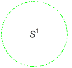
A unit $d-$dimensional sphere is defined such that:
$$ S^d = \left\{ x \in \Bbb{R}^{d+1} : \left \lvert x \right \rvert = 1 \right\} $$
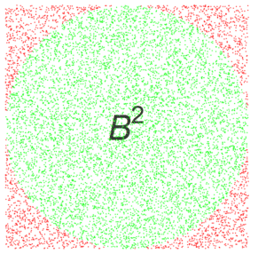
And a unit $d-$dimensional ball is defined such that:
$$ B^d = \left\{ x \in \Bbb{R}^{d} : \left \lvert x \right \rvert \leq 1 \right\} $$
So the perimeter of a circle is a 1-sphere, and the interior of the circle (a disk) is a 2-ball.
And if the earth was perfectly spherical, than the surface of earth would be a 2-sphere, and the interior of the earth would be a 3-ball.
The way I remember these definitions, is that for both the $d$-sphere and the $d$-ball, the $d$ signifies how many degrees of freedom it has.
Uniform Random Sampling
In this post, we adopt the convention that ‘uniform random sampling‘, ‘(continuous) simple random sampling‘, and even ‘uniform sampling‘ are all fully synonymous. And that for discrete probabilities, this means that all possible elements of $S$ have an equal probability of being selected. For continuous probabilities, this means that the likelihood of an element falling in any subinterval is directly proportional to the length of the subinterval.
Virtually all computer languages have a built-in function for this concept. For example , $\text{rand}(\cdot)$, that produces a random number that is (pseudo)-randomly drawn from uniform distribution $[0,1)$.
Note 1.
In contrast to many of my other posts on this blog, we are not talking about quasirandom sampling (aka ‘evenly distributed’), we are just talking about ‘plain old simple vanilla’ uniform random sampling.
Note 2.
For the coding examples, I generally use readable python code (built on numpy), except for acceptance/rejection methods where I used pseudo-code. The purpose of the code is aimed for clarity and so does not necessarily include language-specific conventions or optimizations. It uses the notation that $x**y$ is equal to $x^y$.
Although each of them have their strengths and weaknesses, an asterisk (*) indicates methods that I believe are an excellent default option for that section.
Uniformly sampling a 1-sphere (a circle).
That is, uniformly sampling points on the circumferende of a circle.
*Method 1. Polar
This should be very clear to everyone, and is the foundation for many of the other methods.
theta = 2*PI * random()
x = cos(theta)
y = sin(theta)
Method 2. Rejection Method
A lesser-known method (Cook, 1957) that does not directly require trigonometric functions.
You might notice that the expressions have almost identical structure to Pythagorean triplets!
(This method is better known when generalised to the 2-sphere.)
Select u,v ~ U(-1,1)
d2 = u^2+v^2
If d2 >1 then
    reject and go back to step 1
Else
    x = (u^2-v^2)/d2
    y = (2*u*v)/d2
Return (x,y)
Method 3. Muller , Marsaglia (‘Normalised Gaussians’)
This method was first proposed by Muller and then Marsaglia and the popularised by Knuth, it is very elegant. It naturally generalizes and remains efficient for higher dimensions.
Presumably, it is less well-known due to the less obvious (magical?!) relationship between a circle and the Normal Distribution.
Note that in this version (and its generalizations), the standard deviation does not have to be 1, it just has to be identical for all the random variates. However, in nearly all implementations, a standard error of 1 is picked due to its convenience.
Also, in the absence of a native function, a simple and common method to draw from a normal distribution is via the Box-Mueller algorithm.
u = np.random.normal(0,1)
v = np.random.normal(0,1)
d= (u^2+v^2)**0.5  # notation for sqrt(.)
(x,y) = (u,v)/d
To very briefly understand why this works, consider the function
$$ f(u,v) = f(\mathbf{z}) = \left( \frac{1}{\sqrt{2\pi}} e^{-\frac{1}{2}u^2} \right) \left( \frac{1}{\sqrt{2\pi}} e^{-\frac{1}{2}v^2} \right) $$
After some algebra, this simplifies to
$$ f(u,v) = f(\mathbf{z}) = \left( \frac{1}{(\sqrt{2\pi})^{3/2} }\right) e^{-\frac{1}{2}(u^2+v^2)} = \left( \frac{1}{(\sqrt{2\pi})^{3/2} }\right) e^{-\frac{1}{2}(|\mathbf{z}|^2)} $$
This illustrates that the probability distribution of $\mathbf{z}$ only depends on its magnitude and not any direction. Thus it must be rotationally invariant (symmetric). And thus, must correspond to a uniform distribution on the circle.
This argument is not specific to $d=2$ and can be generalized to any $d$.
Uniformly sampling a 2-ball (disk).
That is, uniformly sampling points inside a circle.
*Method 4. Rejection Method
This is probably the most intuitive method, and is quite fast for a 2-ball.
However, (as discussed later) it generally gets a bad rap, because if you generalize this algorithm to higher dimensions, it can become catastrophically very inefficient.
1. Select x,y ~ U(-1,1)
2. If (x^2+y^2 >1) then reject and go to step 1.
3. Return (x,y)
Method 5. Polar + Radial CDF
For balls of any dimension, a very common method of uniformly picking from a $d$-ball, is to first select a random directional unit-vector from a $(d-1)$-sphere, and then multiply this vector by a scalar radial multiplicative factor.
The crucial aspect of this algorithm is the multiplicative factor, $\sqrt{\cdot}$ function. This is intuitively required because area, which corresponds to the cumulative distribution function (CDF), grows according to $r^2$, so we need to apply the inverse of this. See here for a more visual explanation of this.
The following method is notably asymmetrical. Geometrically, one variable is used for radial distance and the other for the angular displacement.

u = random()
v = random()
r = u**0.5  # sqrt function
theta = 2* PI *v
x = r*cos(theta)
y = r*sin(theta)
*Method 6. Concentric Map (Shirley 1997)
This variance reduction method (Shirley, 1997) is fascinating and motivated by the idea that ideal mappings from the square-based random variate $uv$-space to the coordinate $xy$-space (disks) should be area-preserving, two-way continuous, and with low distortion. By comparing the figures for method 5 and method 6, it should be clear why this one generally produces better results in (finite) MC methods. Additional visual explanation and analysis of this method is given here (which also include some other variations including ‘squircle’, elliptical and approximate equal areas).

u= random()
v = random()
if (u==0 && v==0) return (0,0)
theta=0
r = 1
a=2*u-1
b=2*v-1
if(a*a>b*b)
    {r = a; theta = PI/4*b/a}
else
    {r = b; PI/2- theta /4*a/b}
x= r*cos(theta)
y= r*sin(theta)
Method 7. Muller / Marsaglia (‘Normalized Gaussians’)
This method is a hybrid of methods 3 and 5, because it selects a random direction via method 3 and a random radius via method 5.
u = np.random.normal(0,1)
v = np.random.normal(0,1)
norm = (u*u+v*v)**0.5
r = pow( np.random(0,1),1/2.)
(x,y) = r*(u,v)/norm
Method 8. Exponential Distribution
Another stunningly elegant method (Barthe, 2005) that is valid for balls of any dimension, is to draw $d$ random variates from the normal distribution, and a single random variable from the exponential distribution (with $\lambda=1/2$).
(Note that I believe there is a typo in the original paper, as the original paper says $\lambda = 1$, which has then also been copied into Wolfram’s mathworld.)
Recall, that in the absence of a native function, a simple and common method to draw from an exponential distribution with parameter $\lambda$, is via the negative logarithm of a uniform random variate divided by $\lambda$.
u = np.random.normal(0,1)
v = np.random.normal(0,1)
e = np.random.exponential(0.5)
denom = (u*u + v*v + e)**0.5
(x,y) = (u,v)/denom
Method 9. Dropped Coordinates
A somewhat magical method, first noted by (Harman and Lacko 2010) and then proven ( Voelker 2017) that is not well-known is that if $(x_1,x_2,x_3,x_4)$ is a random vector uniformly distributed on the $3$-sphere, the random vector $(x_1,x_2)$, (that is, with the last two coordinates dropped) is uniformly distributed in the $2$-ball.
See method 20 for a more detailed commentary of this method.
s = np.random.normal(0,1)
t = np.random.normal(0,1)
u = np.random.normal(0,1)
v = np.random.normal(0,1)
norm = (s*s + t*t + u*u + v*v)**(0.5)
(x,y) = (u,v)/norm

Uniformly sampling a 2-sphere (surface of a sphere).
That is, uniformly sampling points on the surface of a sphere.

Method 10. Polar
This is the natural generalization of method 1. Note that the inverse cosine is required for the same reason that the sqrt is required in method 5.
u = random()
v = random()
theta = 2 * PI * u
phi = np.arccos(2v-1)
x   = np.sin(theta) np.cos(phi)
y   = np.sin(theta) np.sin(phi)
z   = np.cos (theta)
Using $u=\cos \theta$, an equivalent version of this that does not directly involve inverse trig functions is
u   = 2*random()-1
phi = 2* PI * random()
x = cos(phi) * (1-z^2)**0.5
y = sin(phi)* (1-z^2)**0.5
z = u
*Method 11. Muller
This is a direct generalization of method 3.
u = np.random.normal(0,1)
v = np.random.normal(0,1)
w = np.random.normal(0,1)
norm = (u*u + v*v + w*w)**(0.5)
(x,y,z) = (u,v,w)/norm
Method 12. Rejection Method #1
This method (Marsaglia, 1972) is a direct generalization of Method 2 .
Select u,v ~ U(-1,1)
d2 = u*u + v*v
If d2>1 then
    reject and go to step 1.
Else
    x = 2*u* sqrt (1-d2)
    y = 2*v* sqrt (1-d2)
    z = 1-2*d2
Return (x,y,z)
Method 13. Rejection Method #2
This method (Cook, 1957) is quite different to any of the previously discussed methods.
For those variables that are accepted, the rules for quaternion transformations, imply that the following points are uniformly distributed.
Select s,t,u,v ~ U(-1,1)
d2 = s^2 + t^2 + u^2 + v^2
If d2>1 then
    reject and go to step 1.
Else
    x = 2*(s*u+t*v)/d2
    y = 2*(u*v-s*t)/d2
    z = (s*s-t*t+u*u-v*v)/d2
Return (x,y,z)
Uniformly sampling a 3-ball (interior of a sphere).
That is, uniformly sampling points on the inside of a sphere.
*Method 14. Rejection Method
This method is a direct generalization of Method 2. Again, it is quite efficient as the acceptance rate is still relatively high and the calculations can be done blazingly fast. However, it carries a bad reputation as it is catastrophically inefficient for higher dimensions.
1. Select x,y,z ~ U(-1,1)
2. If (x^2+y^2 +z^2>1) then reject and go to step 1.
3. Return (x,y,z)

*Method 15. Muller
This is combination of method 7.
u = np.random.normal(0,1)
v = np.random.normal(0,1)
w = np.random.normal(0,1)
r = random()**(1./3)
norm= (u*u+v*v+w*w)**(0.5)
(x,y,z) = r*(u,v,w)/norm
*Method 16. Polar
This is the natural generalization of method 5.
u = 2*random()-1
phi = 2* PI * random()
r = random()**(1/3.)
x = r* cos(phi) * (1-u^2)**0.5
y = r* sin(phi)* (1-u^2)**0.5
z = r*u
Method 17. Exponential Distribution
This is a direct generalisation of method 8. Again, note that I believe there is a typo in the original paper, as the original paper says $\lambda = 1$, which has then also been copied into Wolfram’s mathworld.
u = np.random.normal(0,1)
v = np.random.normal(0,1)
w = np.random.normal(0,1)
e = np.random.exponential(0.5)
denom = (e + u*u + v*v + w*w)**0.5
(x,y,z) = (u,v,w)/denom
Method 18. Dropped Coordinates
A natural extension of method X.
Based on the fact that if $(x_1,x_2,x_3,x_4,x_5)$ is a random vector uniformly distributed on the $4$-sphere, the random vector $(x_1,x_2,x_3)$, (that is, with the last two coordinates dropped) is uniformly distributed in the $3$-ball.
See method 20 for a more detailed commentary of this method.
s = np.random.normal(0,1)
t = np.random.normal(0,1)
u = np.random.normal(0,1)
v = np.random.normal(0,1)
w = np.random.normal(0,1)
norm = (s*s + t*t + u*u + v*v + w*w)**(0.5)
(x,y,z) = (u,v,w)/norm
Uniformly sampling a $d$-sphere.
*Method 19. Muller
For higher dimensions where $d>3$, most of the above methods do not neatly simplify. Therefore, the one that is almost always used for a $d$-sphere is the generalised version of methods 3 and 9.
u = np.random.normal(0,1,d)  # an array of d normally distributed random variables
d=np.sum(u**2) **(0.5)
(x,y,z) = (u,v,w)/d
Uniformly sampling a $d$-ball.
Although the rejection methods 4 and 13 are extremely intuitive and trivially generalise to higher dimensions, one quickly encounters ‘the curse of dimensionality’. As mentioned, for $d=1$ the acceptance rate is $\sim 0.71$, and for $d=2$ the acceptance rate is $\sim 0.52$. Although this might appear inefficient, due to not requiring to calculate any complex functions this is often one of the fastest ways to pick points in a $2-$ball or $3$-ball.
By comparing the hypervolume of a $d$-ball with the enclosing cube, one can deduce that for $d=10$, the acceptance rate is less than 0.0025 and it gets exponentially worse for higher $d$.
*Method 20. Muller
In practice, the almost exclusive method to calculate points inside a $d-$ball is the generalized version of method 14. Namely,
u = np.random.normal(0,1,d)  # an array of d normally distributed random variables
norm=np.sum(u**2) **(0.5)
r = random()**(1.0/d)
x= r*u/norm
Method 21. Exponential Distribution
This is a direct generalisation of method 8 and 16.
x = np.random.normal(0,1,d)
e = np.random.exponential(0.5)
denom = (e + np.sum(u**2))**0.5
(x,y,z) = (u,v,w)/denom
*Method 22. Dropped Coordinates
A very elegant method, first noted by (Harman and Lacko 2010) and then proven ( Voelker 2017) that is not well-known is that if $ (x_1,x_2,x_3,…,x_d,x_{d+1},x_{d+2})$ is a random vector uniformly distributed on the $(d+1)$-sphere, the random vector $ (x_1,x_2,x_3,…,x_d)$, (that is, with the last two coordinates dropped) is uniformly distributed in the $d$-ball.
This is non-trivial result where even developing an intuition is difficult, (even the base case of $d=1$ is not trivial!)
However, it may be interesting/useful to note that an $\exp(1/2)$ variable $Y$ in method 19, has the same distribution as $(Y_1^2+Y_2^2)$ where $Y_1,Y_2$ are standard normal – thus connecting this methods 19 and 20.
Thus,
u = np.random.normal(0,1,d+2)  # an array of (d+2) normally distributed random variables
norm=np.sum(u**2) **(0.5)
u = u/norm
x = u[0:d] #take the first d coordinates
Conclusion
This post gives a comprehensive list of the most frequent and useful methods to uniformly sample from a the surface of a $d$-sphere, an the interior of the $d$-ball.
Many of them are simple and intuitive, whilst others are truly remarkable in their structure.
It is of course, possible to always use the most generalised versions of these formulae as outlined in methods 19-22, but sometimes specialised methods for smaller $d$ may be more efficient and/or amenable to understanding.
***
My name is Dr Martin Roberts, and I’m a freelance Principal Data Science consultant, who loves working at the intersection of maths and computing.
“I transform and modernize organizations through innovative data strategies solutions.”You can contact me through any of these channels.
LinkedIn: https://www.linkedin.com/in/martinroberts/
Twitter: @TechSparx https://twitter.com/TechSparx
email: Martin (at) RobertsAnalytics (dot) com
More details about me can be found here.
Excellent summary and presentation of algorithms. Thank you for this contribution.
my pleasure.