I propose a new algorithm for multi-armed bandits that is fully deterministic, as fast and simple to implement as UCB1, and yet, for a very broad range of practical circumstances empirically outperforms many of the existing industry standard Bernoulli multi-armed bandit policies, including Thompson Sampling and UCB1 and UCB-tuned.
tl;dr: Get a summary of this post via ChatGPT here.
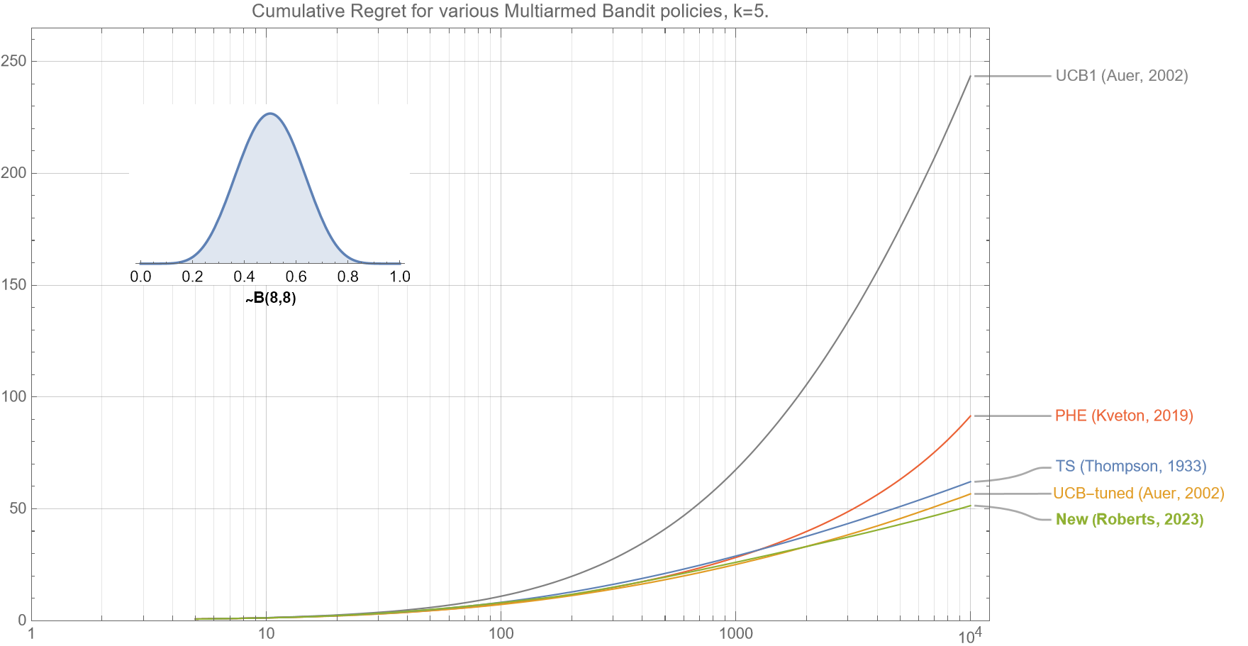
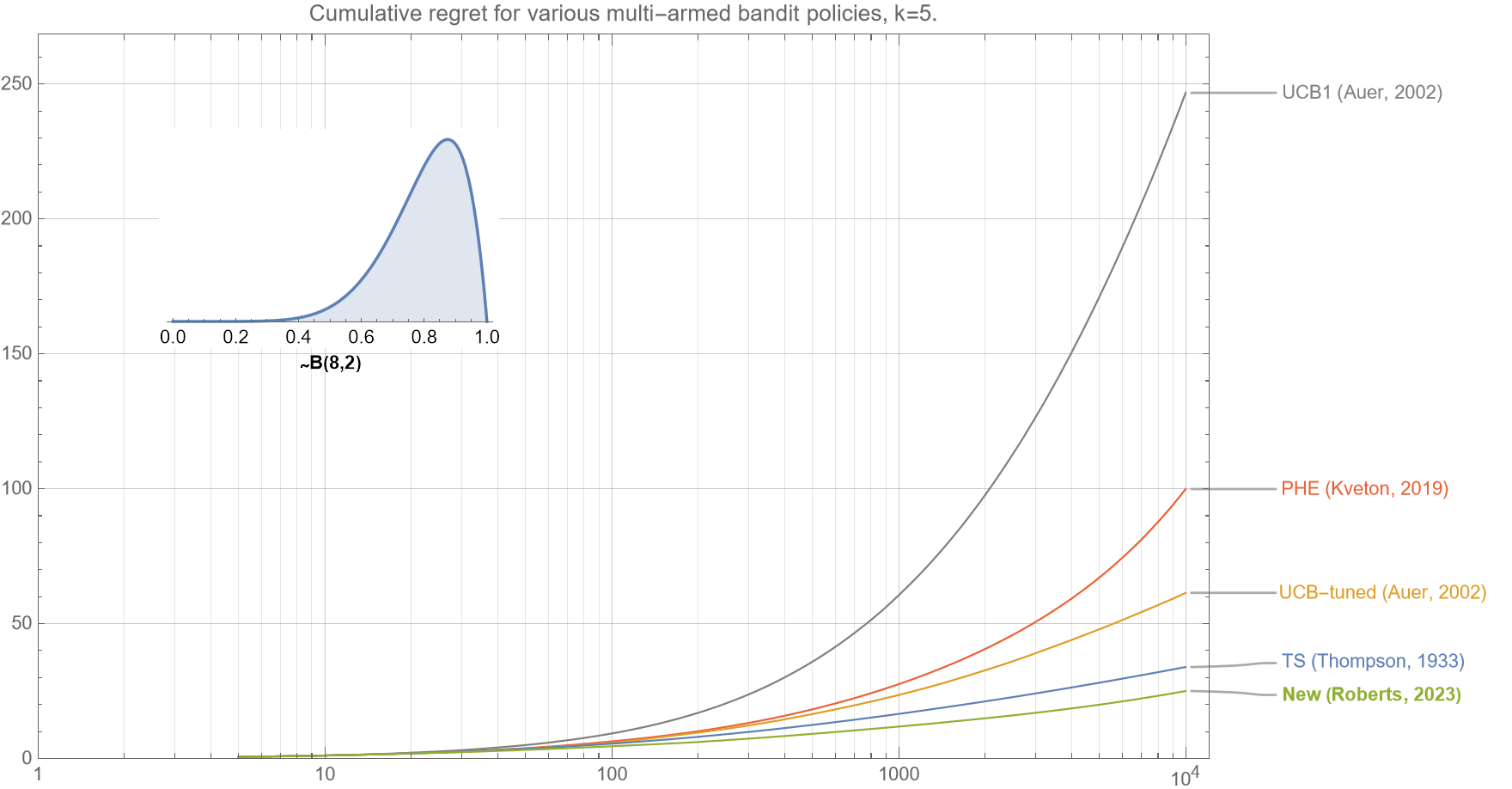
Figure 1. This comparison of various bandit policies shows that if the underlying probabilities for the $k=5$ arms are drawn from a beta distribution $B(8,8)$, then the cumulative regret curve (smaller is better) for our new algorithm (as described in section 2.5) outperforms UCB1, UCB-tuned, Perturbed History Exploration (PHE), and Thompson Sampling for almost all $t<10^4$.
First published: 3 Oct, 2023
Last updated: 24 July, 2025
Section 1. Introduction
Multi-armed bandits are a class of machine learning and optimization problems (which fall in the vategory of active learning / reinforcement learning) that involve making a sequence of decisions in situations where you need to obtain the most out of limited resources despite uncertain outcomes.
The name ‘multi-armed bandits’ and the associated terminology originates from the metaphor that you are in a casino with $k$ slot machines (‘armed bandits) – each with a potentially different payout (probability of giving you a reward). Selecting a particular machine and pulling its arm gives you a reward (or nothing), and your goal is to figure out which machines to play over time to win the most money.
They are used in various fields, including medical research, recommendation systems, clinical trials, resource allocation and robotic systems. For example,
-
-
- Clinical Trials: When testing different treatments for a medical condition, multi-armed bandits can be used to identify the most effective one as quickly as possible, while minimizing patient risk.
- Content Recommendation: Multi-armed bandits can be a powerful tool in content recommendation systems, helping to optimize the selection of content to present to users and improve user engagement.
- Resource Allocation: They can be used to determine how to distribute resources (e.g., customer service agents, server resources) efficiently to maximize outcomes (e.g., customer satisfaction, system performance).
- Robotics and Autonomous Systems: Multi-armed bandits can assist robots to optimally explore their environment and gather information about the world.
-
In essence, multi-armed bandits provide a framework for balancing two primary goals: “Learning and Earning”, or alternatively referred to as “Exploration and Exploitation”.
Learning (‘exploration’) involves trying out different options to learn more about their rewards or outcomes. In the context of multi-armed bandits, it means testing arms (choices) that you have limited information about. Initially, when you have little or no data about the arms, multi-armed bandit algorithms allocate a significant portion of their resources to exploration. This is because you need to gather data to estimate the rewards associated with each arm accurately. During the exploration phase, arms that haven’t been tried much or haven’t shown strong performance in the past are given a chance. This helps reduce uncertainty about their rewards.
Earning (‘exploitation’) involves leveraging your current knowledge to maximize immediate rewards. In the context of multi-armed bandits, it means focusing on arms that are believed to be the best based on the available data. As the multi-armed bandit algorithm collects data and updates its estimates of arm performance, it starts to shift resources toward exploitation. Arms that have demonstrated higher rewards in the past or have more favorable estimates are given priority in recommendations. The exploitation phase aims to maximize the accumulated rewards by recommending arms that are likely to perform well based on historical data.
To balance these two goals effectively, various classes of multi-armed bandit algorithms have been proposed including ε-greedy, Softmax, UCB, Thompson Sampling, Perturbed History Exploration. A brief summary of some of them is as follows.
-
-
- ε-Greedy Strategy. This is a common approach where a small fraction (epsilon, ε) of the time, the algorithm chooses an arm at random (exploration), while the rest of the time, it selects the arm with the highest empirical reward (exploitation).
- Thompson Sampling (TS). This Bayesian approach, first proposed by Thompson (1933), samples from a probability distribution for each arm, that represents both the mean and the uncertainty in their rewards. Arms are chosen based on these samples, favoring arms with higher expected rewards while accounting for uncertainty (exploration).
- Softmax. This algorithm is a probability matching strategy, which means that the probability of each action being chosen is dependent on its estimated probability of being the optimal arm. Specifically, Softmax chooses an action based on the Boltzman distribution for that action. As with the $\epsilon-$greedy strategy, there is typically a tunable parameter $\tau$ that determines the degree of exploration versus exploitation.
- Upper Confidence Bound (UCB) Strategy. This is by far, the most popular and well-studied policy, and was first proposed by Auer et al. (2002). For all algorithms in this class an upper confidence interval for each arm’s reward is estimated. They balance exploration and exploitation by selecting the arm with the highest upper confidence estimate, which accounts for both the mean estimate and an upward bias (exploration) term. Because the bias is always upwards, the UCB algorithms are said to exemplify the principle: “optimism in the face of uncertainty”.
- Perturbed History Exploration (PHE): This lesser-known policy, developed by Kveton et al. (2012) (whilst working in Google’s DeepMind) is an algorithm that adds a number of independent and identically distributed (i.i.d.) pseudo-rewards to the arms’ observations each round, and then pulls the arm with the highest average reward in its perturbed history. The authors describe how (perhaps surprisingly) this algorithm is also consistent with the principle of “optimism in the face of uncertainty”.
-
Some bandit policies are said to be stochastic if there is a degree of randomness in the decision-making at each time step. Thompson Sampling, ε-greedy, Softmax and Perturbed History Exploration are all stochastic algorithms because as part of their decision-making step, they sample from a probability distribution. Specifically:
-
- Thompson sampling samples from a beta distribution.
- ε-greedy samples from a uniform distribution.
- Softmax samples from a weighted uniform distribution
- PHE samples from a binomial distribution
In contrast, if there is no randomness involved in the decision-step, then the algorithm is said to be fully deterministic. A consequence of being fully deterministic, is that they are typically much faster to run as they do not need to draw from particular probability distributions for each arm, at each time, $t$. All the UCB variants, as well as our newly proposed algorithm are fully deterministic.
Regret
Cumulative regret is a key performance metric used in the analysis of multi-armed bandit algorithms. It’s a measure of how much the algorithm potentially loses, by not always choosing the best action. That is, it is the difference between the total reward obtained by the particular bandit policy and the maximum possible cumulative reward that could have potentially been achieved if the best arm had always been selected. A well-performing algorithm will have a lower cumulative regret, indicating that it consistently makes choices that are close to the best possible choices.
Statistically, at each time step $t$, you calculate the regret by taking the difference between the expected reward of the best arm $\mu^*$ and the expected reward of the arm chosen by the algorithm $\mu_{A_j}$. This measures how much better the best arm would have performed compared to the chosen arm at that particular time step. You sum up these regrets over all time steps to get the cumulative regret up to time$t$. That is,
$$ R_t = \sum_t (\mu^* – \mu_{A_t} ) ,$$
where:
$t$ is the total number of time steps or rounds.
$R_t$ is the cumulative regret up to time step $t$
$\mu^*$ is the expected reward of the best arm (the arm with the highest expected reward).
$\mu_{A_t}$ is expected reward of the arm chosen by the algorithm at time step $t$.
Section 2. Multi-armed bandit policies
We give brief descriptions of the common Bernoulli bandit policies and refer the reader to the links at the end of the post for more details. Furthermore, we only discuss and analyse the archetypal multi-armed bandit version, commonly termed the Bernoulli bandit, in which the outcome at each round is only a binary success or fail.
2.1 Upper confidence Bound (UCB1)
- Play each of the $k$ arms exactly once.
- For each round $t>k$, play the action $j$ that maximizes $\hat{x}_j$, where:
$$\hat{x}_j = \bar{x}_j + \sqrt{\frac{2 \ln t}{n_j}} $$
where,
$\bar{x}_j$ is the mean observed reward of arm $j$ after time $t$,
$n_j$ is the number of times that arm $j$ has been chosen so far.
(Intuitively, this formula is just a fancy version of $\hat{x}_j = \bar{x}_j + 2 \sigma $, which is the well-known formula for estimating the 95% upper confidence bound for a Gaussian distribution.)
Interestingly, UCB1 was used as the basis for UBCT, which was a key component of the game engine AlphaGo that famously beat the world champion Lee Sodol, in 2015-16.
2.2 Upper Confidence Bound (UCB-tuned)
- Play each of the $k$ arms exactly once.
- For each round $t>k$, choose the arm $j$ that maximizes $\hat{x}_j$, where:
$$\hat{x}_j= \bar{x}_j + \sqrt{\frac{\ln t}{n_j} \rm{min} \{ \frac{1}{4},V_j \} } $$
where,
$V_j = (\frac{1}{n_j} \sum X^2_j) – \bar{x}^2_j + \sqrt{\frac{2 \ln t}{n_j}}$
Note that the authors use the population (or biased) variance formula. Cursory empirical testing shows that replacing this with the sample (or unbiased) variance formula makes virtually no measurable difference.
2.3 Thompson Sampling (TS)
- For each round $t \geq 1$, choose the arm $j$ that maximises $\hat{x}_j$ where:
$$\hat{x}_{j} \sim B(\alpha+ s_j , \beta + n_j – s_j) $$
where,
$s_{j}$ are the number of successes observed by arm $j$ so far.
$n_j – s_{j}$ are the number of failures observed by arm $j$ so far.
$B(\cdot ,\cdot)$ is the beta distribution function
$B(\alpha ,\beta)$ is a prior, such as $B(1/2,1/2)$ or $B(1,1)$.
2.4 Perturbed History Exploration (PHE)
- Play each of the $k$ arms exactly once.
- For each round $t>k$, choose the arm $j$ that maximizes $\hat{x}_j$, where:
$$\hat{x}_j= \frac{s_j+a_j}{n_j+\lambda n_j} $$
where,
$a_j$ are the number of successes observed in a random trial of $ \lambda n_j$ coin flips.
$ \lambda=1.1$
Recall, that the number of successes from say $m$ coin flips can be obtained sequentially from $m$ observations from a Bernoulli distribution $\sim Ber(0.5)$, or in a single-step via the binomial probability distribution $ \sim Bi(m,0.5)$.
In the paper, the authors show that the algoirthm is asymptotically logarithmic for any $ 1 < \lambda < 2$, and show empirical results using $\lambda= 1.1$.
It is interesting to note that unlike UCB where the bias is always upwards, for PHE this bias for each arm may be upward or downward.
2.5 Our new Algorithm
Note that for the UCB-class of algorithms and the PHE policy, at each time step $t$, the bias varies for each arm. In contrast, for our proposed bandit policy, at each time step, we include the same bias to each arm. Specifically, the bias is equivalent to adding an additional $a$ success outcomes to each arm. That is,
- Play each of the $k$ arms exactly once.
- For each round $t>k$, choose the arm $j$ that maximizes $\hat{x}_j$, where:
$$\hat{x}_j = \frac{s_j+a}{n_j +a } $$where,$s_j$ is the number of successes observed by arm $j$ so far
$u_1 =
\begin{cases}
13, & \text{if $t \leq 150 $ } \\
13 + 8(\ln t -5) , & \text{if $t>150$ }
\end{cases}
$$u_2= \rm{max} \{ \bar{x}_j \} $ for $j=1,2,…,k$.
$a = u_1 \cdot u_2 $
- If two arms have the same pseudo-mean $\hat{x}_j$, then always choose the one with the lowest $n_j$.
In words, our newly proposed policy is as follows:
-
-
- Convert our time into natural logarithmic time.
- Apply a truncated-linear transformation.
- Multiply this result by the observed mean of the currently most successful arm.
- Include this many pseudo-successes to each arm’s observed outcomes.
- Choose the arm with the highest pseudo-mean.
-
Repeating again, the fundamental difference between this policy and UCB, is that for any given time $t$, the bias $a$ is the same for all arms and does not depend on $j$.
Our algorithm is conceptually similar to the UCB algorithms inasmuch as it is fully deterministic and that we add a strictly upward bias factor. However, personally I find that this new algorithm is more similar in nature to Thompson Sampling and PHE. It is similar to Thompson sampling because you can think of the additional $a$ pseudo-observations, acting in a similar manner that a beta prior of $B(\alpha, \beta)$, works for Thompson Sampling.
That is, our algorithm is similar to PHE because in principle, it’s a stochastic policy that samples from the binomial probability distribution $\sim Bi(m,p)$. However, in our case $p=1$. That is, we are interested in the number of successes in a sequence of $m$ Bernoulli trials, each with a corresponding underlying probability of $p=1$. Of course, because a Bernoulli trial with $p=1$ will always succeed, then in practice, this result is fully deterministic!
Note 1. Breaking ties.
Step 3 in the above flow-chart states, “If two arms have the same pseudo-mean $\hat{x}_j$, then always the one with the lowest $n_j$”. A simple and fast way in code to achieve this via code is to modify the maximising function to:
$$\hat{x}_j = \frac{s_j+a+ \epsilon}{n_j +a+\epsilon } $$
where
$\epsilon = 0.001$
For example although $ \frac{15}{50} = \frac{3}{10} $,
$$ \frac{3+\epsilon}{10+\epsilon}= 0.30007 > 0.30001 = \frac{15+\epsilon}{50+\epsilon} $$
Using $2\epsilon$ in the denominator, also works. One might like to think of either of these correction factors as a beta prior of $B(\epsilon,0)$ or $B(\epsilon,\epsilon)$, respectively. Alternatively, one could omit any $\epsilon-$term from the denominator, and this trick would still work.
Note 2. Improved explicit Dependence on $k$
One optimization that can reduce cumulative regret even further (albeit, at the expense of some simplicity) is to replace the constant $t$-intercept term $5$ , in the above formula, with
$t_0 = 3 + \ln (3+k) $
$u_1 =
\begin{cases}
13, & \text{if $t \leq e^{t_0} $ } \\
13 + 8(\ln t -t_0) , & \text{if $t>e^{t_0} $ }
\end{cases}
$
That is,
$ u_1 = 13 +\rm{max} \{ 0, 8 (\ln t – t_0) \} \;\; \rm{for all} \;\; t>k$
For example, for $k=50$ this typically results in about an additional 30% reduction in cumulative regret, compared to simply using $u_0=5$.
Note 3. Finite-horizon correction factor
So far, all the algorithms have been described in their infinite-time form. For the finite-time horizon scenarios where you know that $t$ is bounded by some finite $T$, then we can make the cumulative regret even smaller, by replacing $a= u_1 u_2 $ with the empirical formula:
$$a = u_1 u_2 u_3 $$
where $u_3 = 0.09 \ln T. $
This typically reduces cumulative regret by several percent.
Section 3. Results
3.1 Varying the arms’ underlying reward probability distribution
We first show that our new algorithm empirically consistently outperforms all the other algorithms under a broad range of underlying distributions for the arms’ rewards.
We see in figures 2a-2c, that if the underlying mean rewards for each of the $k$ arms are drawn from a beta distribution $B(8,8)$, then our new policy outperforms all the common existing policies for almost all $t<10^4$.
Note that:
-
- A $~B(8,8)$ is very similar to a Gaussian Distribution $~N(1/2,1/8)$.
- All results have been obtained averaging regret over 10,000 separate runs.
- As the axes for all these plots are log-linear, then a straight-line plot is consistent with logarithmic growth (which can be clearly seen for our algorithm, UCB-tuned, and TS).
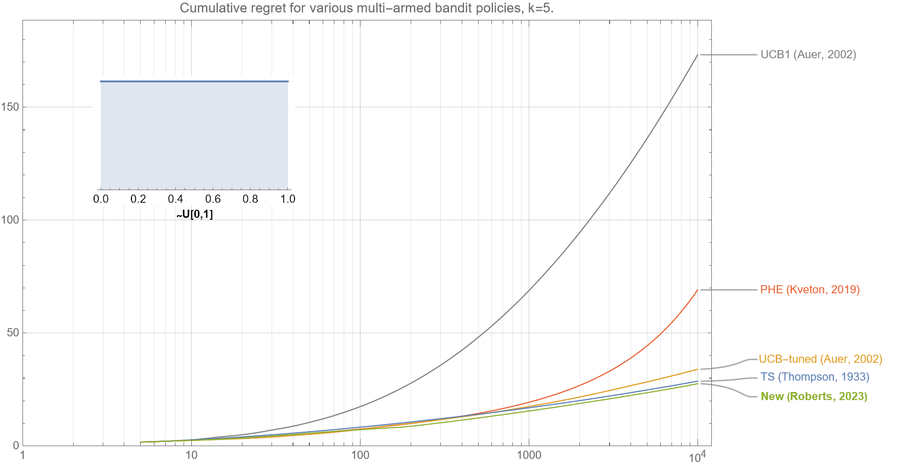
Of interest is that almost identical regret curves for all the policies is obtained if the arms’ underlying rewards $\mu_{k}$ are drawn from the uniform distribution $~U[0.3,0.7]$. Note that for both these distributions, their mean reward and variance is $(\mu, \sigma^2) = (1/2, 0.015)$. This phenomenon is mentioned in reference xx, where they note that regret curves are only dependent on the mean and variance of the underlying distribution and not higher moments.
* * *
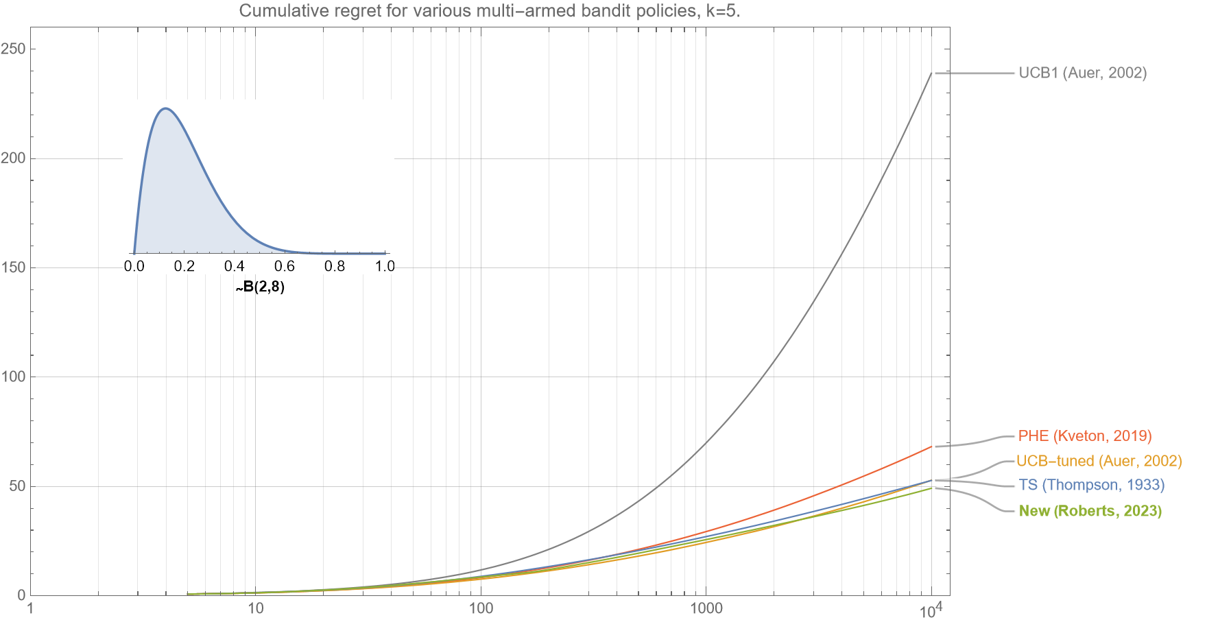
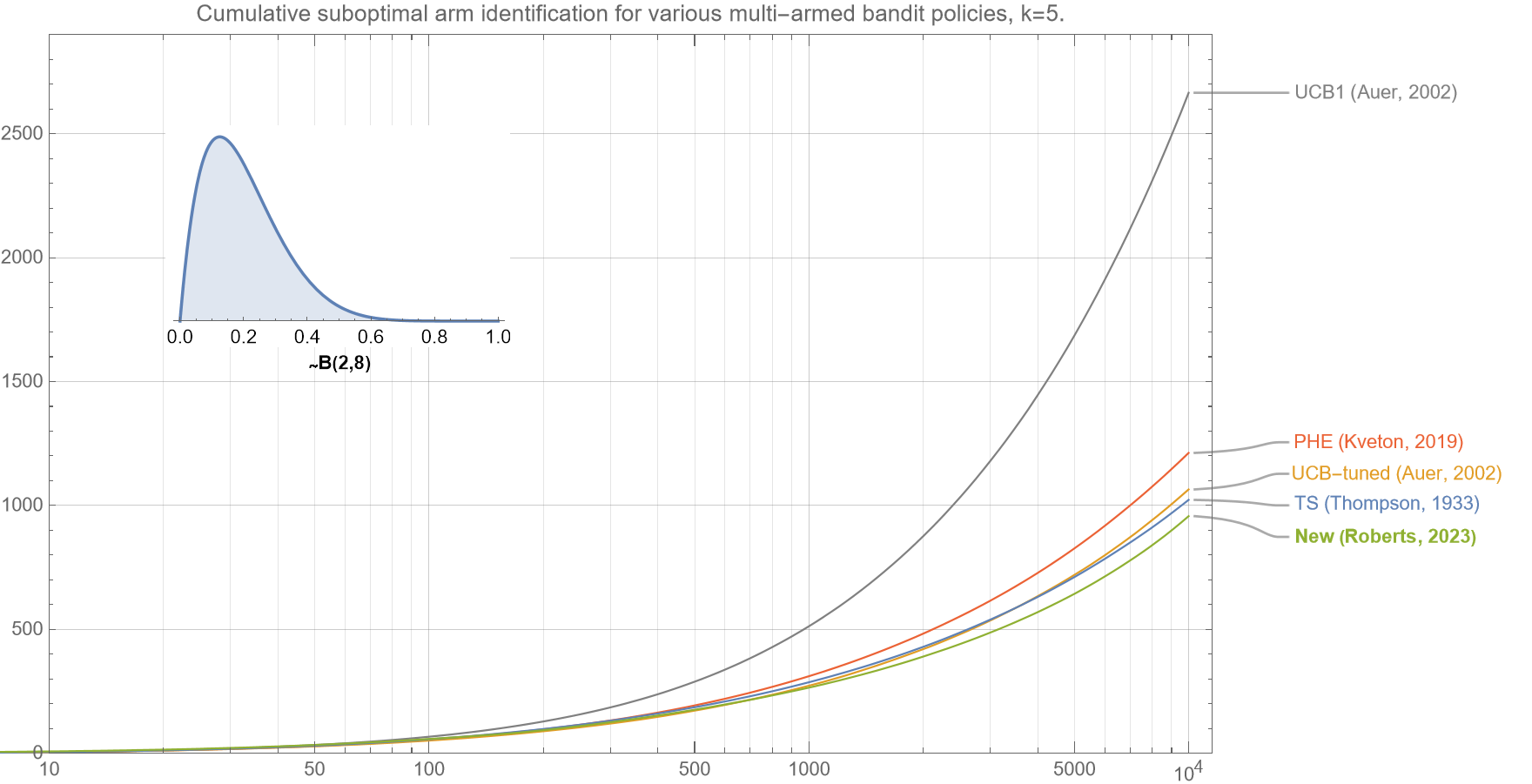
In figure 2d, we see the resulting cumulative regret curves when the underlying mean rewards are drawn from beta distribution $B(2,8)$. This type of distribution is important as it is frequently found in many online digital scenarios where the call-to-action for most arms is quite low, but there is a small chance that one of the arms is highly performant.
In this scenario, the crucial key is that the bandit policy will gain high confidence in the optimal arm as quickly as possible, and only minimal resources are allocated to the suboptimal arms. Again, we see that our new algorithm is: (i) slightly better than Thompson Sampling and UCB-tuned; (ii) significantly better than PHE, and (iii) vastly superior to UCB1, for all $t<10^4$.
Only for scenarios where the mean reward of the optimal arm $\sim 0.5$ does the UCB-tuned outperform our algorithm and Thompson Sampling.
* * *
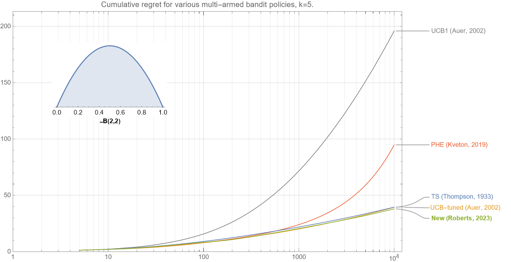
In the following figure (fig. 2e), we see that the cumulative regret curves if the underlying mean rewards are drawn from beta distribution $B(8,2)$. With this type of distribution multiple arms are typically highly performant.
This distribution is of particular interest, as the differential between the optimal arm and the second-best arm is typically very small. In this case, it is important that the policy sufficiently explores the suboptimal arms to ensure that false positives are minimized. Again, we see that our new algorithm is: (i) slightly better than Thompson Sampling, (ii) significantly better than UCB-tuned and PHE, and (iii) vastly superior to UCB1, for all $t<10^4$.
3.2 Varying the number of arms
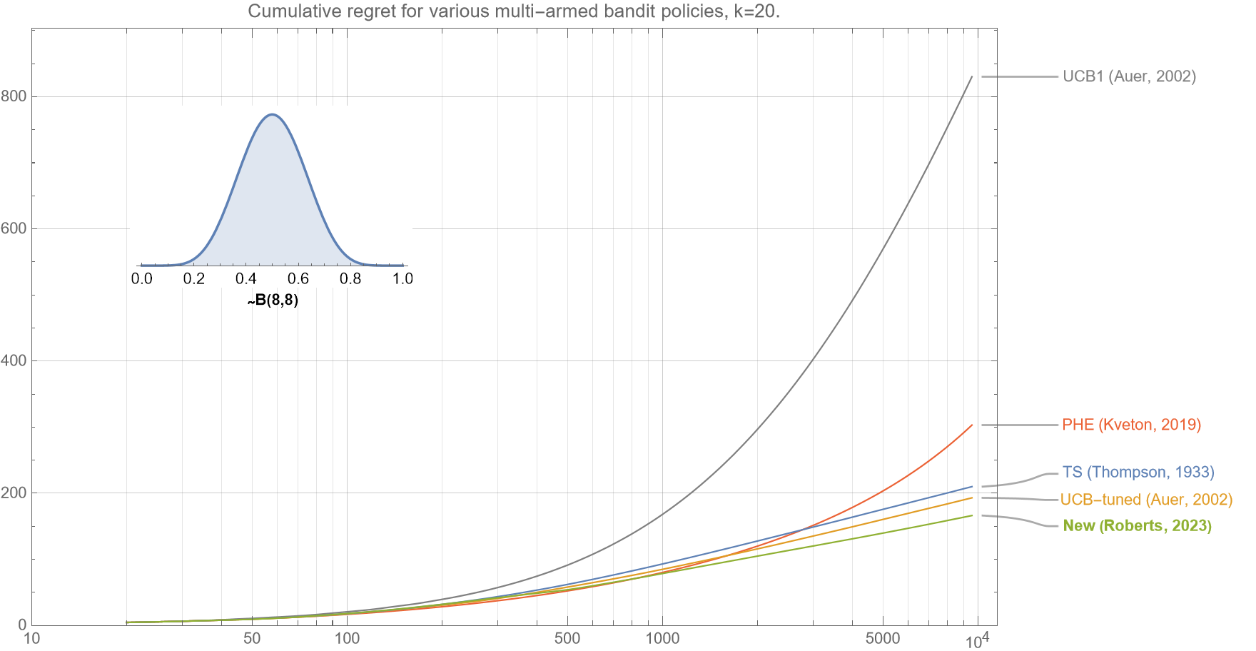
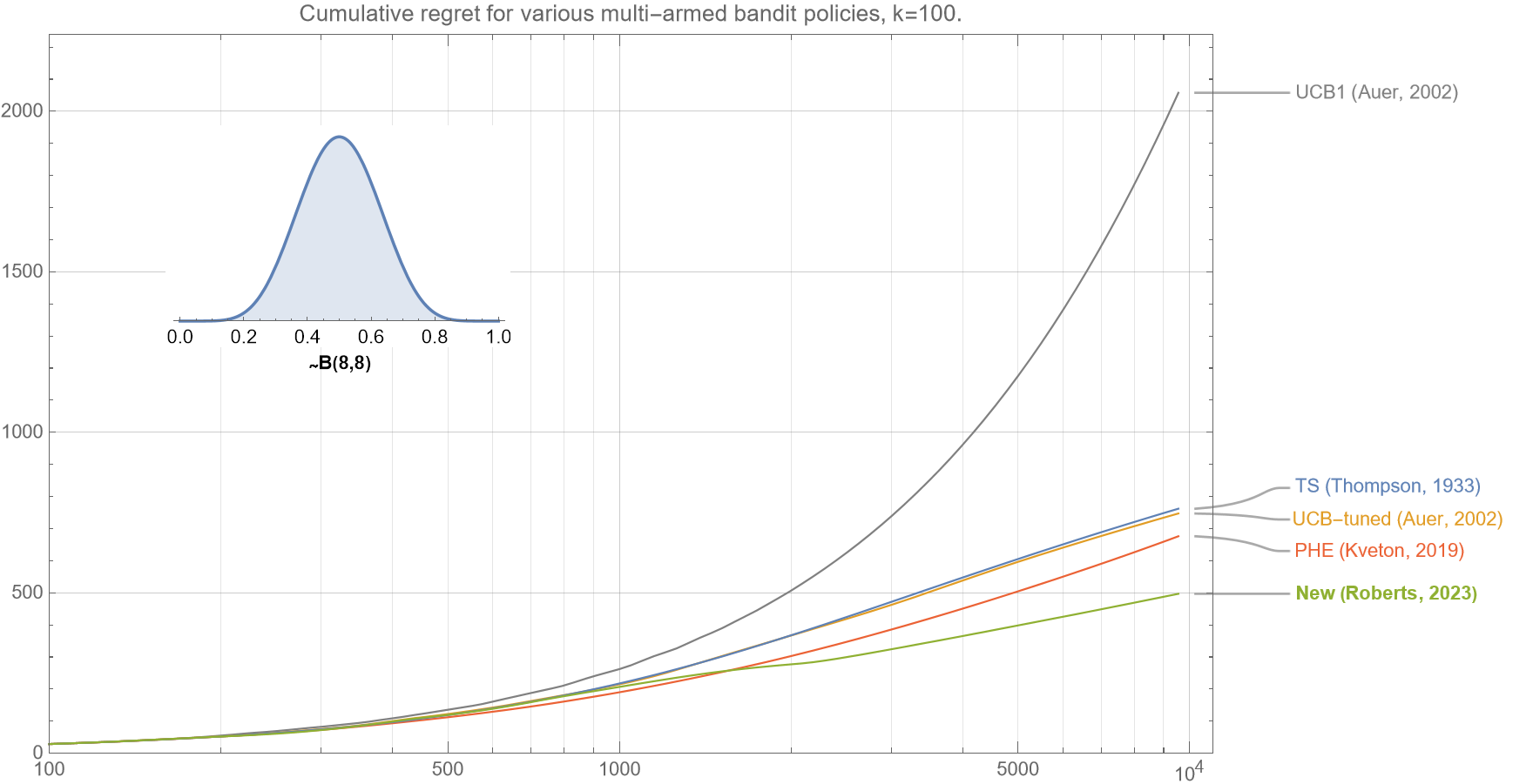
We now show that our new algorithm performs very well across a large range of $k$.
In figures 3a-c, we see that for $k=5,20$, and $100$, the regret curves all show that our new algorithm outperforms all Thompson Sampling, UCB-tuned, PHE and UCB1, for almost all $t<10^4$.
For brevity we only show regret curves associated with $B(8,8)$. Other distributions show similar characteristics (not shown).
Figure 3a (same as figure 1). In this comparison of various bandit policies shows that if the underlying probabilities for the $k=5$ arms are drawn from a beta distribution $B(8,8)$, then the cumulative regret curve (smaller is better) for our new algorithm outperforms UCB1, UCB-tuned, Perturbed History Exploration (PHE), and Thompson Sampling for almost all $t<10^4$.
* * *
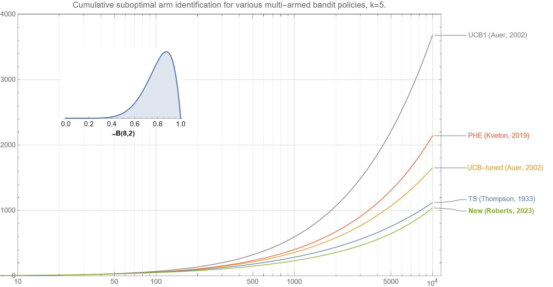
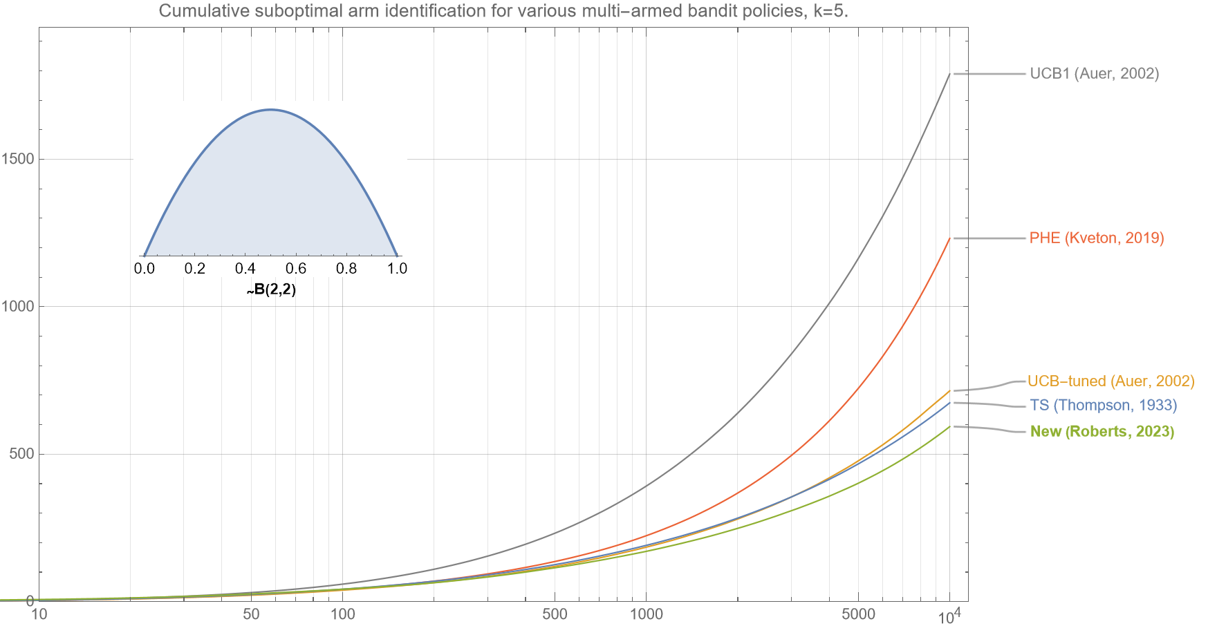
3.3 Suboptimal Arm identification
We now show that our new algorithm correctly identifies the optimal arm more efficiently than existing policies.
Although cumulative regret is the most common metric to optimize for multi-armed bandits, another common metric is how effective they are at identifying the optimal arm. In line with cumulative regret, which actually measures an undesirable quantity and that a lower value is better, the following chart shows ‘cumulative suboptimal arm identification‘ which is the number of times that the bandit algorithm does not select the optimal arm. Similar curves are obtained for other distributions and values of $k$ (not shown).
Note that the axes for figures 4a-4c are log-linear but the curves for almost all the algorithms are not linear but rather upward convex upward, which strongly suggests that the error rate grows faster than logarithmically. Cursory analyses suggests that the identification error for all policies asymptotically grows $\sim \sqrt{t}$.
Section 4. Summary
In this post, I described a new policy for multi-armed bandits. Like UCB1 and UCB-tuned it is fully deterministic and so does not require sampling from any auxiliary probability distributions, and therefore is very fast. It is extremely simple to implement (see section 2.5), and empirical testing shows that it is stable for $t<10^5$, and highly competitive with industry-standard algorithms such as Thompson Sampling, UCB-tuned, UCB1, and PHE for $t<10^4$, for all $k \geq 2$, and across a wide range of underlying reward distributions.
Section 5. Useful links
5.1 Python code repositories ($3^{rd}-$party)
5.2 Blog posts
5.3 Selected papers
Some papers that focus on comparing different multi-armed bandit policies and algorithms:
-
- “A Survey of Online Experiment Design with the Stochastic Multi-Armed Bandit” by Shipra Agrawal and Nikhil Goyal
This comprehensive survey paper discusses various multi-armed bandit algorithms and their applications, providing insights into their comparative performance. - “Empirical Evaluation of Thompson Sampling” by Olivier Cappe, Aurelien Garivier, Emilie Kaufmann, et al.
This paper presents an empirical evaluation of Thompson Sampling, one of the popular multi-armed bandit algorithms, comparing its performance with other algorithms like UCB1. - “Analysis of Thompson Sampling for the Multi-armed Bandit Problem” by S. Agrawal and N. Goyal
This paper delves into Thompson Sampling for multi-armed bandit problems and provides an empirical evaluation of its performance compared to other algorithms. - “The KL-UCB Algorithm for Bounded Stochastic Bandits and Beyond” by Aurélien Garivier and Olivier Cappe
This paper introduces the KL-UCB algorithm, a variant of the UCB algorithm, and empirically compares its performance with other bandit algorithms. - “On Upper-Confidence Bound Policies for Non-Stationary Bandit Problems” by Olivier Cappe, Aurélien Garivier, et al.This paper explores the performance of various Upper Confidence Bound (UCB) policies, including UCB1 and UCB-Tuned, in non-stationary bandit problems.
- “An Empirical Evaluation of Thompson Sampling” by Shipra Agrawal and Nikhil Goyal
This paper provides an empirical analysis of the Thompson Sampling algorithm’s performance in various settings and compares it with other popular bandit algorithms. - “Analyzing Multi-armed Bandit Algorithms” by Xi Chen, Li Chen, and Minghong Lin
This paper offers a theoretical analysis and comparative study of several multi-armed bandit algorithms, including UCB and Thompson Sampling. - “Bayesian Reinforcement Learning: A Survey” by Mohammad Ghavamzadeh, et al.
This survey paper covers various Bayesian reinforcement learning methods, including Thompson Sampling, and discusses their performance in comparison to other approaches. - “Comparing Thompson Sampling and UCB on a Predictive Analytics Task” by Pannaga Shivaswamy, et al.
This paper evaluates Thompson Sampling and UCB in the context of predictive analytics and compares their effectiveness in solving real-world problems.
- “A Survey of Online Experiment Design with the Stochastic Multi-Armed Bandit” by Shipra Agrawal and Nikhil Goyal
***
My name is Dr Martin Roberts, and I’m a Principal Data Science consultant, with international experience and expertise working at the intersection of mathematics and computing.
“I transform and modernize organizations through innovative data strategies solutions.”You can contact me through any of these channels.
LinkedIn: https://www.linkedin.com/in/martinroberts/
email: Martin (at) RobertsAnalytics (dot) com