The Theil-Sen (Kendall) and Siegel estimators are non-parametric distribution-free methods used to fit a line to data, in ways that are very robust to large levels of noise and outliers. We briefly illustrate how the lesser-known Siegel estimator is typically better than the more commonly used Theil-Sen estimator.

First published: 7th March, 2019
Last updated: 26 July, 2020

Introduction

In situations where you know that the (y-value) errors associated with your data are normally distributed, than in almost all cases you should use standard linear least squares regression. However, in situations where either:

- - the errors follow a different (‘fatter tailed’) distribution,
  - some of the errors are outliers

then it is usually better to apply alternative estimators. Two excellent choice are the Theil-Sen (Kendall) estimator and the Siegel Repeated median estimator.

Example I

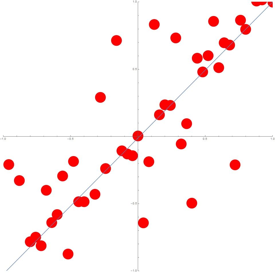
Suppose we consider, $n=50$ data points where the $x_i$ are evenly distributed on the interval $[-1,1]$.

Now consider $y_i = x_i + \epsilon_i$ for all $i$.

Ordinary least squares offers an optimal solution when $\epsilon$ is distributed according to $N(0,\sigma)$. However, suppose in this case it is actually distributed according to something more extreme such as $\left[ U(-1,1) \right]^3$.

In this case, the data could typically look like this:

Least-Squares

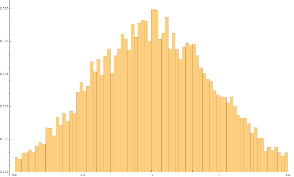
Typically, the slope of a line is estimated using least-squares.

If we run say $m=10^4$ trials, we find that using Least-Squares, the expected slope is 1.0 with an MSE of 0.0085.

The fact that the mean slope is essentially 1 is reminder that this estimator is unbiased.

Theil-Sen (Kendall) Estimator

The famous Thiel-Sen esimator (1950), (also often called the Kendall estimator due to its relationship with the Kendall tau-rank correlation coefficient) and then calculates the slope of the line according to:

$$ m = \text{median} \left\{ \frac{y_i-y_j}{x_i-x_j} \right\} \quad\text{for all } i \neq j $$

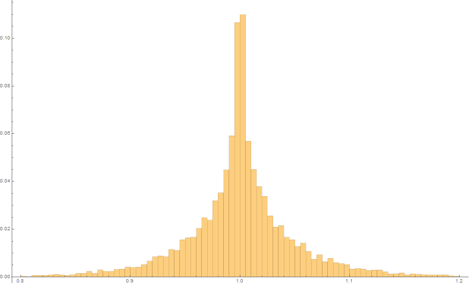
We can understand the slope distribution associated with this formula by simulating say $m=10^4$ trials.

We find that again the expected slope is 1.0, but this time with an MSE is only 0.0025!

So we an an unbiased estimator that typically has a variance over three times lower!

This method typically offers better results than standard linear regression, for $n>6$.

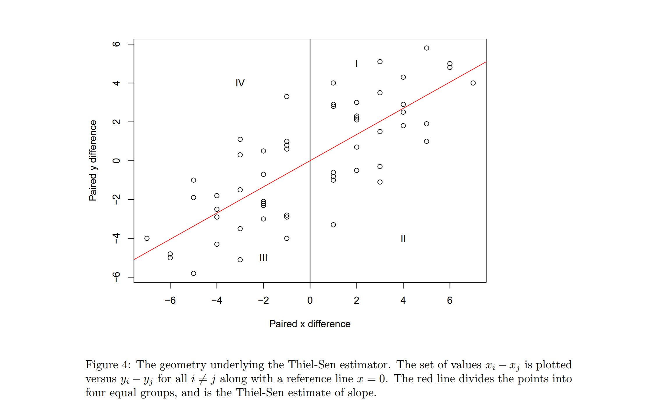
As an aside, the following diagram might assist in developing a stronger intuition on Theil-Sen regression line. (source: cran.r-project.org).

The estimator equally partitions the $(x,y)$- differences into four equal count regions.

Figure 3b. A geometric understanding of the Theil-Sen estimator.

Siegel’s Repeated Median Estimator

A lesser-used variant of this is Siegel’s Repeated median estimator (1982), which is generally more robust and typically has even less variance.

For each point $(x_i,y_i)$, the median of all the slopes $(y_j − y_i)/(x_j − x_i)$ of lines through that point is calculated, and then median of each of these means is calculated. Not only is this theoretically more robust to outliers, it generally produces an even lower variance in slope esimates.

$$ m = \begin{matrix} \text{median} \\ i \\ \end{matrix} \left( \begin{matrix} \text{median} \\ j\neq i \\ \end{matrix} \left\{ \frac{y_i-y_j}{x_i-x_j} \right\} \right)$$

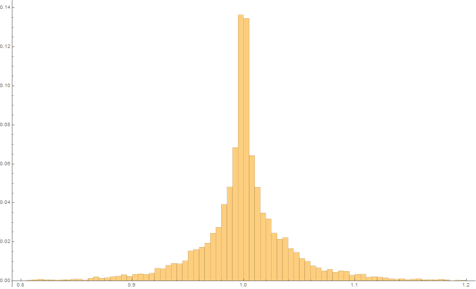
In this case, $m=1000$ trials produces an expected slope of 1.0 but an MSE of only 0.0015, which is about two-thirds the variance of the Theil-Sen estimator, and five times less than the least-squares method.

Siegel’s repeated median estimator typically offers better results than the Thiel-Sen, for $n>14$.

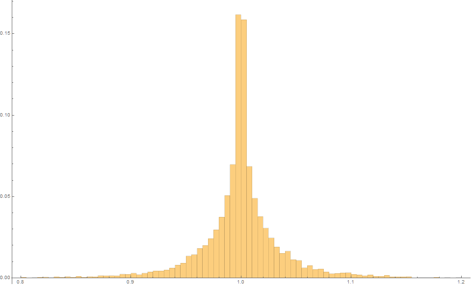
Example 2.

Suppose we consider, $n=50$ data points where the $x_i$ are (uniformly) randomly distributed on the interval $[-1,1]$.

Again, suppose $y_i = x_i + \epsilon_i$ for all $i$, and that $\epsilon \sim \left[ U(-1,1) \right]^3$.

In this case, the data could typically look like this:

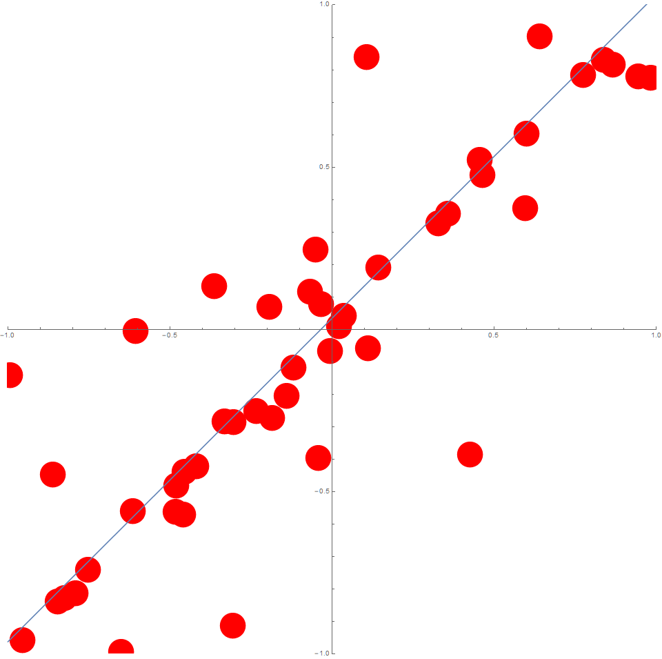
*Figure 5. Typical Data with random $x_i$.*

The Least squares estimator produces an expected estimate of 1.0 with an MSE of 0.0089

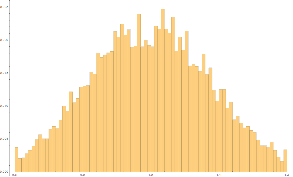
*Figure 6. Least Squares estimator with random $x_i$.*

The Theil-Sen estimator produces an expected estimate of 1.0 with an MSE of 0.0028

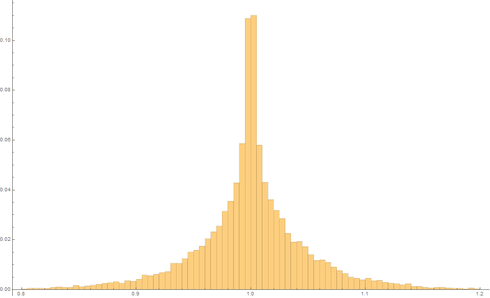
*Figure 7. Theil-Sen estimator with random $x_i$.*

And finally, the Siegel estimator produces an expected estimate of 1.0 with an MSE of just 0.0020

Figure 8. Siegel estimator with random $x_i$.

Conclusion

These two simple examples illustrate that although the Theil-Sen estimator is far more well known, and often cited as ‘the most popular non-parametric technique for estimating a linear trend‘, the more recent proposed “Siegel Repeated Median estimator” is typically more robust unbiased estimator with generally lower variance for $n>14$.

***

My name is Dr Martin Roberts, and I’m a freelance Principal Data Science consultant, who loves working at the intersection of maths and computing.

“I transform and modernize organizations through innovative data strategies solutions.”
You can contact me through any of these channels.
LinkedIn: https://www.linkedin.com/in/martinroberts/
Twitter: @TechSparx https://twitter.com/TechSparx
email: Martin (at) RobertsAnalytics (dot) com
More details about me can be found here.

The Theil-Sen and Siegel non-parametric estimators
for linear regression