Most two dimensional quasirandom methods focus on sampling over a unit square. However, sampling evenly over the triangle is also very important in computer graphics. Therefore, I describe a simple and direct construction method for a point sequence to evenly cover an arbitrary shaped triangle.
Outline
Low discrepancy sequences that evenly sample/cover a square have been extensively studied for nearly a hundred years. Most of these quasirandom sequences can be extended to rectangles by simple dilation without much deterioration of discrepancy.
However, this post looks at the interesting and important extension of low discrepancy sequences over an arbitrary triangle.
As far as I can deduce, very little work has been done on constructing evenly distributed points sets and sequences over triangles. Notable efforts in recent years by Basu [2014] and Pillands and Cools, [2005] and Brandolini [2013] represent the main papers – if not the only papers on this subject. For a post on Basu’s approach when applied to graphics rendering, see here.
These authors generally take a very theoretical and analytical approach to this issue and almost solely focus on either the regular or right-angled triangle/simplex. In contrast, this post is mainly intended to aid in the development of some practical techniques for graphics rendering.
This post describes a simple and direct method that requires no acceptance/rejection, no dropping or recursion; and most importantly it can be applied to triangles of arbitrary shape and size.
This post has four sections
- Quasirandom Sequences in the square
- Mapping the unit square to a triangle.
- Reducing Aliasing
- Further generalizations
1. Quasirandom Point Sequences
You might think it is easy to place 100 points in a square such that the minimum distance between neighboring points is as large possible. But what if you had to place 13 points? 47? … or how about 2019 points?!
It turns out that low discrepancy point sequences offer a systematic way to solve this problem. There are many low discrepancy quasirandom sequences including the simple Halton sequence to the more sophisticated Sobol’ sequence. Each of these particular sequences have their advantages and disadvantages. For example, Halton sequences tend to be more useful when placing objects in a region, as the local distance metrics such as nearest neighbor are well optimized. In contrast, the Sobol’ sequence tends to have more ‘clumping’, however, its global point distribution is very even, and so it has excellent quadrature properties.
There is another sequence I love to use, which has both excellent local as well as global properties. This is the $R_2$ sequence, as described in detail in my other post, “The Unreasonable effectiveness of Quasirandom Sequences”.
In brief, we define the infinite two-dimensional sequence $R_2$, such that
$$ \pmb{t}_n = \left\{ n \pmb{\alpha} \right\} \quad n=1,2,3,… $$
$$ \textrm{where} \quad \pmb{\alpha} =\left(\frac{1}{g}, \frac{1}{g^2} \right), $$
$$ \textrm{and} \; g \simeq 1.32471795572 \tag{1}$$
More details on this special value of $g$, which is often called the ‘plastic constant’ can be found on Wikipedia or Mathworld.
In summary, figure 2 shows a comparison of various low discrepancy sequences (and simple uniform random sampling for comparison). You can see, that random sampling exhibits clustering of points and that there are also regions that contain no points at all (‘white noise’), whereas a low discrepancy sequence quasirandom sequence is a method of constructing an (infinite) sequence points in a deterministic manner such that, at any stage, the placed points are evenly distributed across the entire space.
2. Mapping the unit square to a triangle.
There are three well known methods to allow one to uniformly random sample from a triangle. These are:
- the Parallelogram method ,
- the Kraemer Method and
- the inverse cumulative distribution method.
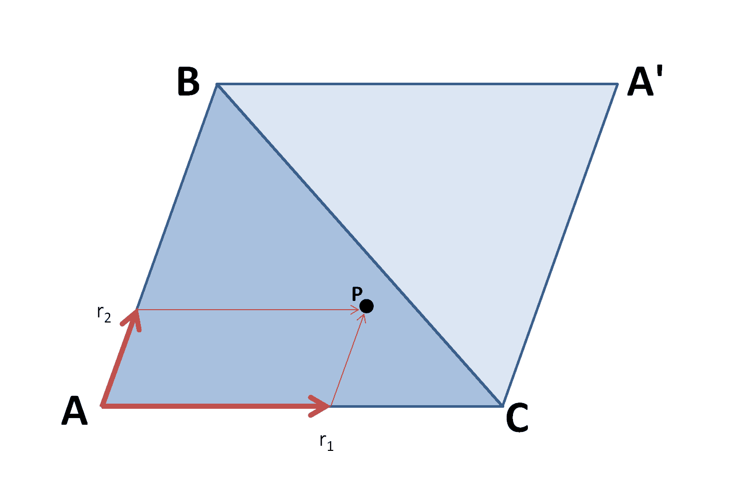
The parallelogram method is as follows.
For a triangle $\pmb{ABC}$, consider the parallelogram $\pmb{ABCA’}$.
For a point in the unit square $(r_1,r_2)$, define the point $\pmb{P} $ such that $ \pmb{P} = r_1 \pmb{AC} + r_2 \pmb{AB} $.
This point will always fall inside the parallelogram. However, if it occurs in the complementary triangle $\pmb{ABC’}$, then we need to reflect it back into the triangle $\pmb{ABC}$.
That is, if $r_1+r_2<1$, then $ \pmb{P} = r_1 \pmb{AC} + r_2 \pmb{AB} $, but if $r_1+r_2>1$, then $ \pmb{P} = (1-r_1) \pmb{AC} + (1-r_2) \pmb{AB} $.
However, it is very important to understand that just because these methods allow uniform sampling from a triangle, this does not imply that such a transform will preserve the even spacing (ie low discrepancy) of our quasirandom point distributions.
For example, for the parallelogram method, the reflection may frequently cause a point to be placed very close to another existing point. This obviously breaks the critical low discrepancy structure and the effect will be appear as aliasing/banding.
Similarly the inverse cumulative distribution method applies a non-linear distortion to the points. For the Halton and Sobol sequences this means that frequently two points are pushed very close to each other.
Figure 3 shows how well the low discrepancy is preserved for each of the different quasirandom sequences when you transform the region from a unit square to a triangle using the parallelogram method.
Of the three different methods to triangulate, and the numerous different quasirandom sequences to choose from, the parallelogram method applied to the $R_2$ sequence method is the only combination that consistently produces acceptable results in terms of preserving low discrepancy without aliasing.
The excellent results of this combination can be further seen in figure 4.
3. Other considerations
Aliasing.
The parallelogram method requires selecting two sides of the triangle to be picked as the basis vectors.
If the vertices are labelled in a random order, then the point patterns are typically as seen in figure 5.
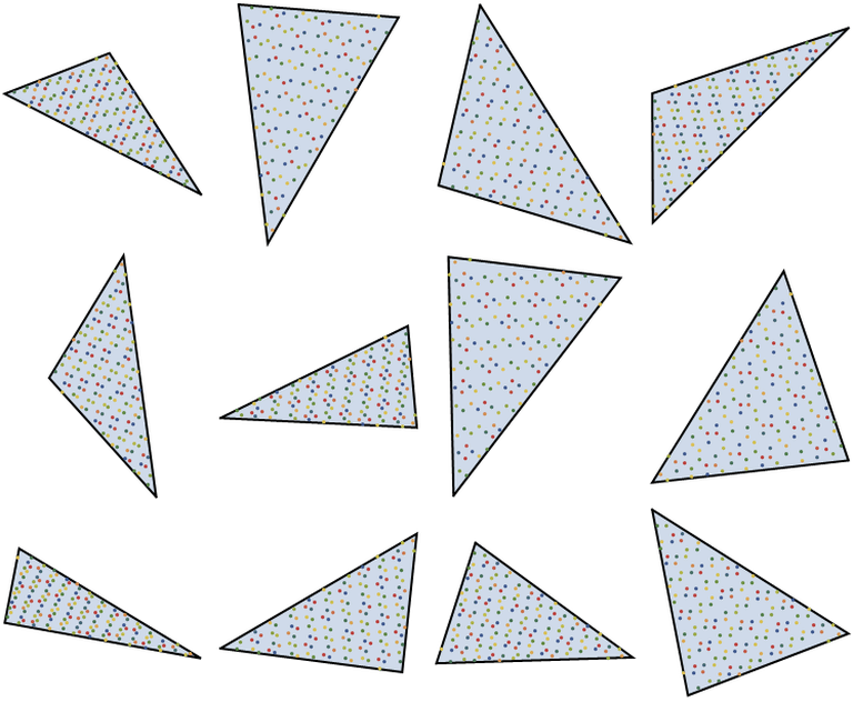
However, it turns out that a judicious choice of vertex ordering, allows aliasing to be significantly minimized. Most notably, if the triangle is labelled such that $A$ is the largest angle (and thus opposite the largest side), and thus the two sides $\pmb{AB}$ and $\pmb{AC}$ are used for the two sides of the parallelogram.
If this protocol is adopted, then the resulting point patterns can be seen in figures 1, 3 and 4 above.
However, even with the particular ordering of vertices, aliasing effects can still be seen in some instances. These are most noticeable when in triangles when one of the angles is small. For obtuse angles, if the smallest angle is less than 30 degrees, some aliasing is visible, and for acute triangles, if the smallest angles is less than 20 degrees aliasing becomes visible. (If the triangles to sampled are part of a Delaunay mesh, then these aliasing issues may be minimal, as Delaunay triangulation is specifically designed to minimize the existence of small-angled triangles.)
Other shapes.
Unfortunately the parallelogram technique can not be used for other shapes, as it exploits the symmetry of the triangle. For some shapes, it is possible to get good results using the inverse cumulative distribution technique. This method is briefly described.
If we revisit figure 3, we can define point P in a manner that guarantees that it will always be inside the triangle, and therefore not require reflecting. Namely, we define $\pmb{P} $ such that
$ \pmb{P} = r_2 \sqrt{r_1} \pmb{AC} + (1-r_2) \sqrt{r1} \pmb{AB} $.
This additional $\sqrt{r_1}$ term not only ensures that the point $P$ always lies inside the triangle, but also (more importantly) that the sampling is uniform. Note that the square root is required because we need an area-preserving transformation, and area increases according to length squared.
More formally, the fractional distance to move in the direction of $\pmb{AB}$ decreases linearly from $z = 1$ to $z=0$. Thus, the cumulative fractional distance is $\int_0^1 z dx = z^2/2$, which is a function of $z^2$, and thus the inverse of this is proportional to $\sqrt{z}$.
Similarly, if we are now attempting to sample from an arbitrary shaped function, we need to use the inverse of the cumulative distribution function. Below is an example of how the $R_2$ low discrepancy sequence can be transformed onto the area bounded under the Gaussian curve whilst generally preserving even spacing between points.
In this case, let $g(z)$ be the inverse cumulative distribution function of the Normal Gaussian function. The then points $P$ will be defined as $$p(r_1,r_2) = \left( g(r_1), r_2 f (g(r_1)) \right ) $$.
If you use the inverse CDF method, it is often best to used a jittered version of a low discrepancy sequence to minmize aliasing. In the example below, i used a jittered version of $R_2$ with a jitter parameter of 0.5. (see “A simple method to construct isotropic quasirandom blue noise“).
***
Thank you to Sergeij Reich for his valuable discussion and analysis on an earlier version of this post.
My name is Martin Roberts. I have a PhD in theoretical physics. I love maths and computing. I’m open to new opportunities – consulting, contract or full-time – so let’s have a chat on how we can work together!
Come follow me on Twitter: @Techsparx!
My other contact details can be found here.
Nice writeup, Ive enjoyed your other posts as well.
I’ve tried the same approach a while ago but found that generating a point inside a parallelogram and mirroring along diagonal if it’s outside of the triangle gives better results (it’s not the same as the Kramer method), at least visually.
There are three problems with the Fibonacci lattice that make it worse:
1. The aliasing is non uniform.
2. The order in which points are added forms streaks of empty space if the number of points used is not just right.
3. When a large number of points is used empty undersampled spots form even for well shaped triangles.
Here is a comparison using the R2 sequence and no jittering, there are 5000 points in the large and 1000 points in the thin triangles:
https://i.imgur.com/2Mh4xLj.png
Even though the parallelogram method has pretty much the same problems as the Fibonacci lattice, they aren’t as severe.
The points are added in an order that gives a better distribution and even mirroring along the diagonal still gives points that are nicely distributed without as noticeable of a pattern. Aliasing is still a problem for sliver triangles of course.
I’ve tried to sort the input coordinates for both methods and while it gives better results, the biggest problems still remain.
Even picking the best of the possible permutations still doesn’t fix it.
I though about using the ratio between the long and short edges of the triangle to skew the points in order to reduce aliasing, but couldn’t find a way of making it work, maybe you have an idea 🙂
So in the end I still don’t have a method that works well for arbitrary triangles, or am I missing something?
Thanks so much for this analysis. Somehow, my early findings showed that the parallelogram method was not great, but it seems that I should not have dismissed the parallelogram method so quickly!
I have come to the same conclusions as you, namely:
(i) sorting the coordinates can make minor/moderate improvements, but for some triangles even the best permutation is bad.
(ii) small angled-triangles notoriously produce signficant aliasing.
But in the end, I also came to the same conclusion as you, that despite these problems, i don’t know of any alternate direct construction methods.
I am thinking the key to your solution is picking points in a parallelogram in a manner that is regular. What method did you use?
I Used Method 2 described in “Generating Random Points in Triangles” by Greg Turk published in Graphics Gems 1.
But here is my code (hope C is not a problem):
https://gist.github.com/sergof/136f84d7ca6f54e8e977d4bd7084b356
The supergolden ratio seems to work just as well as the plastic constant.
That’s very interesting. I’ll try to make mention of this in my follow-up post which is nearly complete. 😉
Any idea how do I add random seed value to this R2 sequence, so that two same triangles could have different point placement, but still using r2 sequence? Can algorithm from this post be implemented in opensource app?
Hi,
It is very easy to incorporate a seed $\pmb{s}$ into the algorithm, so that you can construct a family of different R_2 sequences.
$$ \pmb{t}_n = \left\{\pmb{s}+ n \pmb{\alpha} \right\} \quad n=1,2,3,… $$
where $\pmb{s}$ is any 2-d point in $[0,1] \times [0,1]$.
That is what I tried to do but adding offset to 2d sequence breaks the ‘even distribution’ of points. Below is my test, where I add ‘rand_offset’ 2d point, to the sequence:
https://i.imgur.com/eF1u9ze.gifv
Resulting points do not look uniform for lots of rand_offset values. Unless seed is (0,0) or (0.5, 0.5) – those seems work perfect, but this gives only 2 seed values. Maybe I’m doing something wrong.
Ok, I think I figured this out. Problem is that in Parallelogram method , the points that are outside triangle, should not be moved it the same direction, by seed, as the points in the triangle. I will try to figure way to flip those points seed offset direction somehow.
Hmmm..that’s no good. ☹️
I’ll try to look at it tonight and email you if i figure anything out before you. ?
For now I just ignore points that are oustide triangle (r1+r2>1), that removes half of points, so I just increase target point count two times to compensate. I haven’t figured out better way to negate the random seed offset influence on points distribution.
Regarding the sampling of a triangle, there is a short technical report by Eric Heitz (https://hal.archives-ouvertes.fr/hal-02073696) that gives a area preserving mapping from the square to the cube that seems to have all the required properties regarding the distortion minimization and that is really easy to implement.
His mapping was inspired by the Shirley-Chiu mapping from the square to the disk.
That would allow to use any square sampling pattern to sample the triangle with a minimal loss of sampling quality.
Nice work by the way.
I tested the last page function from Eric Heitz PDF and while it works good with offset, it dosen’t work to well for some number of points, for other it gives visible banding:
https://i.imgur.com/egxcSsc.gifv
I published my way as it offered a method with less banding than any other method I knew about.
So as soon as I/we can fix the offset problem it will certainly be the first choice for triangular sampling.
😉