In this brief post, I describes various methods to estimate uncertainty levels associated with numerical approximations of integrals based on quasirandom Monte Carlo (QMC) methods.

Note

This is a minor follow-up post to the feature article: “The unreasonable effectiveness of quasirandom sequences.”

Topics Covered

• Accuracy of quasirandom monte carlo methods compared to conventional MC methods
• Visualizing uncertainty
• rQMC: Estimating uncertainty via bootstrapping
• Estimating uncertainty via parameterisation
• Estimating uncertainty via cumulative sets
• QMC integration in higher dimensions

Quasirandom Monte Carlo methods for Numerical Integration

Consider the task of evaluating the definite integral

$$A={\int }_0^{1}f(x)\text{d}x$$

We may approximate this by:

$$A\simeq A_n=\frac{1}{n}\sum _{i=1}^{n}f(x_i),x_i\in [0,1]$$

• If the $\{x_i\}$ are equal to  $i/n$, this is the rectangle rule;
• If the $\{x_i\}$ are chosen randomly, this is the Monte Carlo method; and
• If the $\{x_i\}$ are elements of a low discrepancy sequence, this is the quasi-Monte Carlo method.

This post considers two low discrepancy sequences: the (base 2) Van der Corput sequence and the $R({\varphi }_d)$ , defined as:

$${\mathbf{t}}_n=[{\alpha }_0{\alpha }_0+n\alpha \alpha ],n=1,2,3,\dots$$

$$\text{where}\alpha \alpha =(\frac{1}{{\varphi }_d},\frac{1}{{\varphi }_d^2},\frac{1}{{\varphi }_d^3},\dots \frac{1}{{\varphi }_d^d}),$$

$$\text{and}{\varphi }_d\text{is the smallest value of }x>0\text{such that}$$

$$x^{d+1}=x+1.$$

Further information on this newly proposed $R({\varphi }_d)$-sequence can be found on the post “The unreasonable effectiveness of quasirandom sequences“.

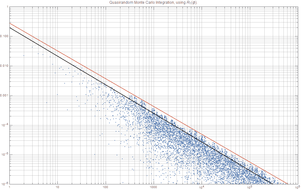
Figure 1 shows the typical error curves $s_n=|A-A_n|$ for approximating a definite integral associated with the function, $f(x)=\text{exp}(-x^2/2),x\in [0,1]$ with: (i) quasi-random points based on the $R(\varphi )$, (blue);(ii) quasi-random points based on the van der Corput sequence, (orange); (iii) randomly selected points, (green). It shows that for $n={10}^6$ points, the random sampling approach results in an error of $\simeq {10}^{-4}$, the van der Corput sequence results in an error of $\simeq {10}^{-6}$, whilst the $R(\varphi )$-sequence results in an error of $\sim {10}^{-7}$, which is $\sim$10x better than the van der Corput error and $\sim$ 1000x better than standard uniform random sampling.

Several things from figure 1 are worth noting:

• This figure illustrates the well known results that (for fixed $d$), the errors based on uniform random sampling asymptotically tend to $1\sqrt{n}$, whereas errors based on quasi-random sequences tend to  $1/n$.
• The van der Corput sequence offers incredibly consistent results for integration problems – that is, extremely low variance!
• The  $R(\varphi )$-sequence produces more accurate estimates, but with greater variance. However, the worst approximations are still comparable to the best approximations of the van der Corput sequence.
• A small variation in the number of sampling points /(n/), for the $R(\varphi )$ sequence typically results in a significantly different level of accuracy.

This last point is the focus of this article. Namely,

For a given number of sampling points $n$, how can we determine the level of confidence / uncertainty  associated with an approximation based on quasi-random Monte Carlo (QMC) methods?

Unlike standard random sequences that are typically used, the accuracy of a quasirandom simulations (such as those based on the Van der Corput / Halton sequences) cannot be as easily calculate or even estimated using the sample variance of the evaluations or by bootstrapping. This article explores some possible solutions to this, as well as suggesting why quasi Monte Carlo methods based on the newly proposed $R(\varphi )$ quasirandom sequence offers some benefits that contemporary low discrepancy sequences do not possess.

Let’s initially focus on the error estimates associated with the $R(\varphi )$-sequence. Looking at figure 2, intuitively, one expects that we could replace the blue point-based estimates, with a line/curve that represents a represents a smoother relationship between $n$ and the estimated error.There are a few possibilities for what that line might look like.

If one wishes to find an upper bounded approximation to the integral, then one would expect that our line would look similar to the red line, and if one wanted a expected estimate that minimized some norm (say, L1 or L2) one would expect the line to look something like the black line in figure 2. This post explores how we might calculate such lines. (Note that since figure 2 is a log-log plot, the black line is closer to the top of the blue dots, than the middle of them).

 

Randomized Quasi-Monte Carlo Methods: (rQMC) Basic Bootstrapping

Suppose we wish to find the uncertainty associated with an estimate based on  $n=1000$ points.

From figure 2 alone,  one might expect that for n=1000, the error would may be be around 0.0002  (black line) but possible as high as  0.0004  (red).

A basic bootstrapping approach would be to take the set $S$, of the all the function values calculated at each of the $n=1000$ points as defined by $R(\varphi )$, and then to take various samples of size $m$ from S and then from each these calculate $k$ different bootstrapped approximations to $A_n$.

That is, define $S$ as follows:

$$R(\varphi ):\{x_i\}=0.618034,0.236068,0.854102,0.472136,0.0901699,0.708204,0.326238,0.944272,0.562306,0.18034,\dots$$

$$S:\{f(x_i)\}=0.826147,0.972521,0.694374,0.894531,0.995943,0.778196,0.948176,0.640296,0.85377,0.98387,\dots$$

The two most common sampling approaches are to either:

1. Create $k$ bootstrapped sets, each with  $m=n$ elements from S, based on sampling with replacement, or
2. Create $k$ bootstrapped sets, each with $m=n/2$ elements from S,  based on sampling without replacement.

Remembering that in practice, where $f$ is a complex function the initial calculation of $f$ at each the $n=1000$ points that is resource-intensive, but the the post-bootstrapping sampling process is extremely light.

The distribution of $k={10}^6$ bootstrapped estimates based on these two methods is shown in figure 3.

 

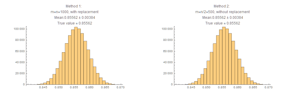
Several things to note about figure 3:

1. Both methods give very virtually identical results for the estimated mean, and standard deviation .
   (For those experienced with bootstrapping, this is actually to be expected, but still often worth explicitly showing.)
2. Both give an estimate of the mean which is within 0.00001 of the true value, and yet the uncertainty implied via the standard deviation is 0.00380.
3. This 95% upper bound for the error is close to 0.008, which is considerably higher than figure 2 suggests.

That is, estimates based on these bootstrapped methods suggest a level of uncertainty much greater than the point estimates indicate in figure 2!

Based solely on this one example, this incredible precision may be attributed to just ‘good luck’ and a value slightly different to n=1000, may result in a much worse error estimate. However, a further explorations (not shown in this posts) show that the uncertainty implied by the standard deviation is consistently much greater than the actual accuracy of the estimates)

The Koksma-Hlawka inequality offers a clue as to why these estimates may not necessarily match what we expected from figure 2. The Koksma-Hlakwka inequality states that:

$$|A_n–\int f(u)du|=|\frac{1}{n}\sum f(x_i)–\int f(u)du|\le V(f).D_n^{\ast }(x_i)$$

What this means, is that the error associated with integral approximations based on quasi random sequences can be (completely) separated into an uncertainty purely associated with the function $f$, and an uncertainty purely associated with the set $x_i$! This truly amazing inequality offers a sound theoretical upper bound on the error. However, in practice if often offers very little clue about the size of the actual uncertainty as it seems that in many instances actual errors can be far smaller than this upper bound indicates.

With this inequality, in hand, we can now think that the uncertainty analysis based on these bootstrapped methods, is more associated with the function, rather than the actual choice of $\{x_i\}$. Thus, it is now a little clearer why standard bootstrapping is not an effective tool for determining confidence levels of approximants based on quasirandom sequences.

Independent Approximations: via Cranley-Patterson rotations.

Like the previous method, this method employs creating $k$ different estimates. However, unlike the previous method,  where the bootstraps were synthetically created and were each approximants of $A_n$, this approach requires independently calculating $k$ different exact values of $A_n$. Thus, this is not bagging – (bootstrap aggregating). That is, although this method is not practical due to being resource intensive, it may offer insight into the underlying uncertainty levels.

Recall that the low discrepancy $R$-Sequence, which is defined at the start of this article, includes a single adjustable parameter, ${\alpha }_0$. In one dimension, this is a single real-valued number. It should be clear that different values of $alph{a}_0$ will not affect the structure or global characteristics of this sequence. This is in direct contrast to many other low discrepancy sequences where the parameters often have very large effects. For example, the (2,3)-Halton sequence shows quite distinct differences to the (2,5)-Halton sequence. The fact that only the addtive recurrent low discrepancy sequences have this characteristics, is why this method is not directly applicable for the commonly used low discrepancy sequences such as Halton, Sobol or Faure!

This suggests that by calculating the integral approximants for $n=1000$, multiple times each time with a different values of ${\alpha }_0$ may give us insight into the underlying uncertainty levels.

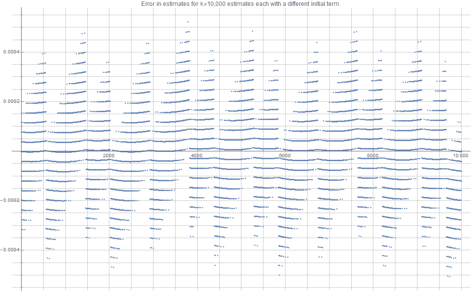
Figure 4 indicates that the error estimates associate with $k={10}^4$ trials, each with a different value of ${\alpha }_0.$ For each trial $i=1,2,3,\dots ,k;\text{let}{\alpha }_0=i/k$. The fact that it appears that this function is equally above and below the axis, is consistent with principles that if ${\alpha }_0$ is chosen randomly, that it would results in an unbiased estimate..

However, more importantly we find that the standard deviation of these $k$  estimates is 0.00017. This suggests an upper 95% confidence error bound of 0.00034.

This seems a lot closer to intuitive expectations than the previously variance estimates based on standard bootstrapping.

 

 

Independent Approximations – higher dimensions

The previous method works for higher dimensions, too. It just requires the selection of k different starting seeds chosen from $[0,1{)}^d$. (Uniform sampling is one option, but so is quasirandom sampling!)

There is, however, also another method of finding $k$ different exact estimates for d>1.

Suppose, d=6. Then recall that  $\alpha \alpha =({\alpha }_1,{\alpha }_2,{\alpha }_3,{\alpha }_4,{\alpha }_5,{\alpha }_6)$  where $alph{a}_i=1/{\varphi }^i$.

Then another way of calculating an exact value of $A_n$ is by rearranging the order of the components, that is say , ${\alpha }^{\prime }{\alpha }^{\prime }=({\alpha }_3,{\alpha }_5,{\alpha }_1,{\alpha }_6,{\alpha }_2,{\alpha }_4)$.

This method offers $k=6!=720$ different ways of calculating $A_n$. This new sequence $R^{\prime }(\varphi )$ is a $d$-dimensional rotation of the original sequence, $R(\varphi )$.

Note that this rearranging of the order of components, is fundamentally different to the scrambling techniques often used to construct higher dimensional low discrepancy sequences – where the order of the terms are rearranged.

 

Cumulative Approximations

If we are willing to accept a slightly lower level of independence, we can achieve an approximation to that achieved with the independent approximations method, but with far less resourcing.

Suppose we define, $A_n^{[j]}$ such that $A_n^{[j]}=\frac{1}{n}\sum f(x_i);i=j,j+1,j+2,,,,n+j-1$.

Clearly,  $A_n^{[1]}$ corresponds to our standard value of $A_n$.

This way, the sequence $\{A_n^{[j]}\},j=1,2,3,\dots k$ represents $k$ separate estimates, each based on a different (but not independent) seed.

For k=40, one can infer that the expected estimate is $0.85555\pm 0.00010$. Note that:

• the true value 0.85562 falls within this 68% confidence interval of  $x\in [0.85545,0.85565]$
• the upper bound of the 95% confidence interval suggests an upper bound error of ~ 0.00020
• this uncertainty estimate is consistent with the previous method of independent approximates.

Recall that although it is typically expensive to calculate $f$, one does not need to run the entire analysis 40 times to use this method. You just need to do calculate $f$ for the for first $n=1040$ and then take $k$ consecutive subsets of length $n$ to determine the approximants. Furthermore, obviously, one can choose a different width other than $k=40$. Interestingly, the calculated uncertainty is very robust/smooth to this width.For example, for $k=200$ results in an almost identical standard deviation of 0.00012.

One can realise that if we since we are using an additive recurrence model, taking progressive / consecutive subsequences is equivalent to selecting the sequence of seed values ${\alpha }_0$ for each samples to be simply an arithmetic progression.

Furthermore, this method can work for any approximant that is based on an extensible low-discrepancy sequence. This includes the additive recurrence sequences, and Halton sequences, but not the lattices.

The simplicity, robustness, computational efficiency and generalized applicability of this final method, would suggest that with all other things being equal, this is the preferred method to estimate underlying uncertainties.

 

Key References

• [Snyder, 2000]
• [owen, 2008]
•  [Kolenikov, 2007] (paper);  [Kolenikov, 2007] (talk)
• [Taytaud, 2006]

 

Other Posts you might like:

• Evenly Distributing Points in a Triangle
• The Unreasonable Effectiveness of Quasirandom Sequences.
• Evenly distributing points on a sphere
• A simple method to construct isotropic quasirandom blue noise point sequences
• Going Beyond the Golden ratio