How to distribute points on the surface of a sphere as evenly as possibly is an incredibly important problem in maths, science and computing, and mapping the Fibonacci lattice onto the surface of a sphere via equal-area projection is an extremely fast and effective approximate method to achieve this. I show that with only minor modifications it can be made even better.

First published: 10 August, 2018
Last modified: 7 June , 2020

 

***

This post has been superceded by the more recent post:

“How to evenly distribute points on a sphere more evenly than the canonical Fibonacci Lattice“

Please reference this newer link wherever possible.
This post has been kept as an archival record.

***

A while back, this post was featured on the front page of Hacker News. Visit here for discussion.

Introduction

The problem of how to evenly distribute points on a sphere has a very long history and is one of the most studied problems in the mathematical literature associated with spherical geometry. It is of critical importance in many areas of mathematics, physics, chemistry including  numerical analysis, approximation theory, coding theory, crystallography, electrostatics, computer graphics, viral morphology to name just a few.

Unfortunately, with the exception of a few special cases (namely the platonic solids) it is not possible to exactly equally distribute points on the sphere. Furthermore, the solution to this problem is critically dependent on the criteria used to judge the uniformity. There are many criteria in use, and they  include:

• Packing and covering
• Convex hulls, Voronoi cells and Delaunay  triangles,
• Riesz $s$-energy kernels
• Cubature and Determinants

Repeating this point as it is crucial: there is usually no single optimal solution  to this question, because an optimal solution based on one criteria is often not an optimal point distribution for another.  For example, in this post, we will also find that optimising for packing does not necessarily produce an optimal convex hull, and vice-versa.

For sake of brevity, this post focuses on just two of these: the minimum packing distance and convex hull / Delaunay mesh measures (volume and area).

Section 1 will show how we can modify the canonical Fibonacci lattice to consistently produce a tighter packing configuration.

Section 2 will show how we can modify the canonical Fibonacci lattice that produce larger convex hull measures (volume and surface area).

Section 1. Optimizing Packing Distance

This is often referred to as “Tammes’s problem” due to the botanist Tammes, who searched for an explanation of the surface structure of pollen grains. The packing criterion asks us to maximize the smallest neighboring distance among the $N$ points. That is,

$$d_N=\underset{i\ne j}{min}\Vert x_i–x_j{\Vert }_2$$

This value decreases at a rate ~$1/\sqrt{N}$, so it is useful to define the normalized distance, and also the asymptotic limit of the normalized distance as

$$d_N^{\ast }=\sqrt{N}{d}_N,d^{\ast }=\underset{N\to \mathrm{\infty }}{lim}{d}_N^{\ast }$$

The Fibonacci Lattice

One very elegant solution is modeled after nodes appearing in nature such as the seed distribution on the head of a sunflower or a pine cone, a phenomenon known as spiral phyllotaxis. Coxeter demonstrated these arrangements are fundamentally related to the Fibonacci sequence, $F_k=\{1,1,2,3,5,8,13,\dots \}$ and the golden ratio $\varphi =(1+\sqrt{5})/2$.

There are two similar definitions of the spherical Fibonacci lattice point set in the literature. The original one is strictly only defined for $N$ equal to one of the terms of the Fibonacci sequence, $F_m$ and is very well studied in number theory.

$$t_i=(\frac{i}{F_m},\frac{i{F}_{m-1}}{F_m})\text{for }0\le i\le N-1$$

Whilst the second one generalises this to arbitrary $N$, and is used more frequently in computing:

$$\begin{array}{}\text{(1)}& t_i=(\frac{i}{N},\frac{i}{\varphi })\text{for }0\le i\le N\end{array}$$

where

$$\varphi =\frac{1+\sqrt{5}}{2}=\underset{n\to \mathrm{\infty }}{lim}\left(\frac{F_{n+1}}{F_n}\right)$$

The spherical fibonacci spiral produced from equation 1, results in a value of $d_N^{\ast }$ for all $N$, and so $d^{\ast }=2$.

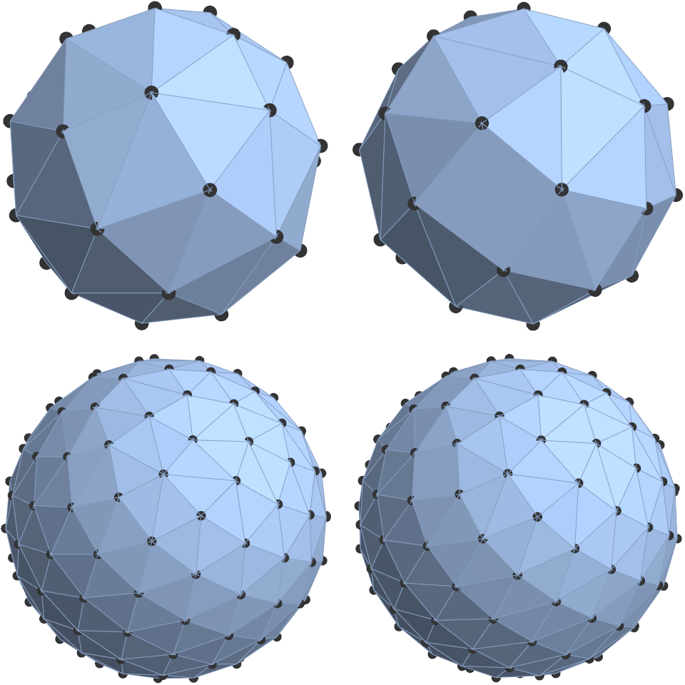
An example of these Fibonacci Grids is shown below. These points sets can be transformed to a well-known Fibonacci spirals via the transformation

$$(r,\theta )=(\sqrt{x_1},2\pi x_2)$$

 

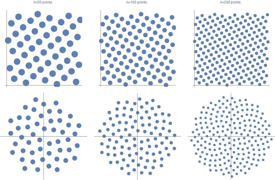
Similarly, these point sets can be mapped from the unit square $[0,1{]}^2$ which to the sphere by the cylindrical equal area projection:

$$(x,y)\to (\theta ,\varphi ):({\cos }^{-1}(2x-1)–\pi /2,2\pi y)$$

$$(\theta ,\varphi )\to (x,y,z):(\cos \theta \cos \varphi ,\cos \theta \sin \varphi ,\sin \theta )$$

Here’s a basic implementation of this in Python.

from numpy import arange, pi, sin, cos, arccos
n = 50
i = arange(0, n, dtype=float) + 0.5
phi = arccos(1 - 2*i/n)
goldenRatio = (1 + 5**0.5)/2
theta = 2 pi * i / goldenRatio
x, y, z = cos(theta) * sin(phi), sin(theta) * sin(phi), cos(phi);

Even though spherical Fibonacci point sets are not the globally best distribution of samples on a sphere, (because their solutions do not coincide with the platonic solids for $n=4,6,8,12,20$), they yield excellent sampling properties and are extremely simple to construct in contrast to other more sophisticated spherical sampling schemes.

As the mapping from the unit square to the surface of the sphere is done via an area-preserving projection, one can expect that if the original points are evenly distributed then they will also quite well evenly distributed on the sphere’s surface. However, this does not mean that it is provably optimal.

This mapping suffers from two distinct but inter-related problems.

The first is that this mapping is area-preserving, not distance preserving. Given that in our case, our objective constraint is maximizing the minimum pairwise distance separation between points, then it is not guaranteed that such distance-based constraints and relationships will hold after the projection.

The second, and from a pragmatic point of view possibly the trickiest to resolve, is that the mapping has a two singularity points at each pole. Consider two points very close to the pole but 180 degrees different in longitude. On the unit square, (and also on the cylindrical projection) they would correspond to two points that are quite distant from each other, and yet when mapped to the surface of the sphere they could be joined be a very small great arc going over the north pole. It is this particular issue that makes many of the spiral mappings sub-optimal.

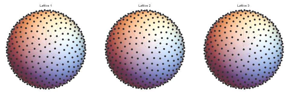
Lattice 1

A common variant, which produces a better packing ($d^{\ast }=3.09$), is:

$$\begin{array}{}\text{(2)}& t_i=(\frac{i+0.5}{N},\frac{i}{\varphi })\text{for }0\le i\le N-1\end{array}$$

It places the points in the midpoints of the intervals (aka the midpoint rule in gausssian quadrature), and so for $n=100$, the values of the first coordinate would simply be:

$$\{\frac{0.5}{100},\frac{1.5}{100},\frac{2.5}{100},\dots ,\frac{97.5}{100},\frac{98.5}{100},\frac{99.5}{100}\}$$

Lattice 2.

A key insight to further improving on Equation 2, is to realize that the $d_N^{\ast }$ always corresponds to the distance between the points $t_0$ and $t_3$, which are at the poles. Thus, to improve $d_N$ the points near the poles should be positioned farther apart.

Let’s define the following distribution:
$$t_i(\epsilon )=(\frac{i+\epsilon }{N-1+2\epsilon },\frac{i}{\varphi })\text{for }0\le i\le N-1$$

Note that $\epsilon =\frac{1}{2}$ corresponds to lattice #1, and a value greater than $\frac{1}{2}$ represents a gap near the poles.

Based on this model, it can be shown that  for $N\ge 20$, compared to the canonical spherical Fibonacci lattice,  the following simple expression corresponding to $\epsilon =\frac{3}{2}$ produces a even better packing ($d^{\ast }=3.27$):

$$\begin{array}{}\text{(3)}& t_i=(\frac{i+1.5}{N+3},\frac{i}{\varphi })\text{for }0\le i\le N-1\end{array}$$

Thus for $N=100$, the values of the first coordinate would simply be:

$$\{\frac{1.5}{103},\frac{2.5}{103},\frac{3.5}{103},\dots ,\frac{98.5}{103},\frac{99.5}{103},\frac{100.5}{103}\}$$

Lattice 3.

As stated earlier, one of the greatest challenges of the distributing points evenly on the sphere is that the optimal distribution critically depends on which objective function you use. It turns out that local measures such as $d_N^{\ast }$ are at times very “unforgiving” inasmuch as a single point in a suboptimal position can catastrophically reduce measure of the entire point distribution.

In our case, regardless of how large $N$ is, the $d_N^{\ast }$ is typically determined by the four points closest to each pole, especially $t_0$ and $t_3$. However, what is also known about this lattice is that the largest Voronoi polygon is at the pole. Thus, in trying to maximize $d_N$ by separating the initial polar points in the sequence, actually makes the void at the pole even larger!  Thus, we present an alternative to lattice 2 which is generally more preferable, as it does not exhibit such a large void near the poles.

It is almost identical to lattice 2 but with two differences. Firstly, it uses $\epsilon =\frac{7}{2}$ for $1\le i\le N-2$. Secondly, in addition to these $N-2$ points, the first and final points are defined to be at located each pole. That is,

$$\begin{array}{}\text{(4)}& t_0=(0,0);t_{N-1}=(1,0);t_i=(\frac{i+3.5}{N+6},\frac{i}{\varphi })\text{for }1\le i\le N-2\end{array}$$
This lattice results in $d^{\ast }=3.313$, which for $N>90$ is even better than lattice #2.

Thus for $N=100$, the values of the first coordinate would simply be:

$$\{0;\frac{3.5}{106},\frac{4.5}{106},\frac{5.5}{106},\dots ,\frac{99.5}{106},\frac{100.5}{106},\frac{101.5}{106};1\}$$

Comparison

For large $N$ this value of $d^{\ast }=3.35$ compares extremely well compared to other methods, such as geodesic domes, which are based on triangulated projections from the faces of platonic solids to the surface of the sphere.

Here are the corresponding values of $d^{\ast }$ for various $N$-point geodesic domes based on the icosahedron.

$$\begin{array}{|ccccccccccc|}\hline N& 12& 42& 92& 162& 252& 362& 492& 642& 812& 1002\\ d^{\ast }& 3.64& 3.54& 3.34& 3.22& 3.15& 3.09& 3.06& 3.03& 3.00& 2.99\\ \hline\end{array}$$

And here are the corresponding values of $d^{\ast }$ for various $N$-point geodesic domes based on the dodecahedron.

$$\begin{array}{|cccccccc|}\hline N& 20& 32& 122& 272& 482& 752& 1082\\ d^{\ast }& 3.19& 3.63& 3.16& 2.99& 2.90& 2.84& 2.81\\ \hline\end{array}$$

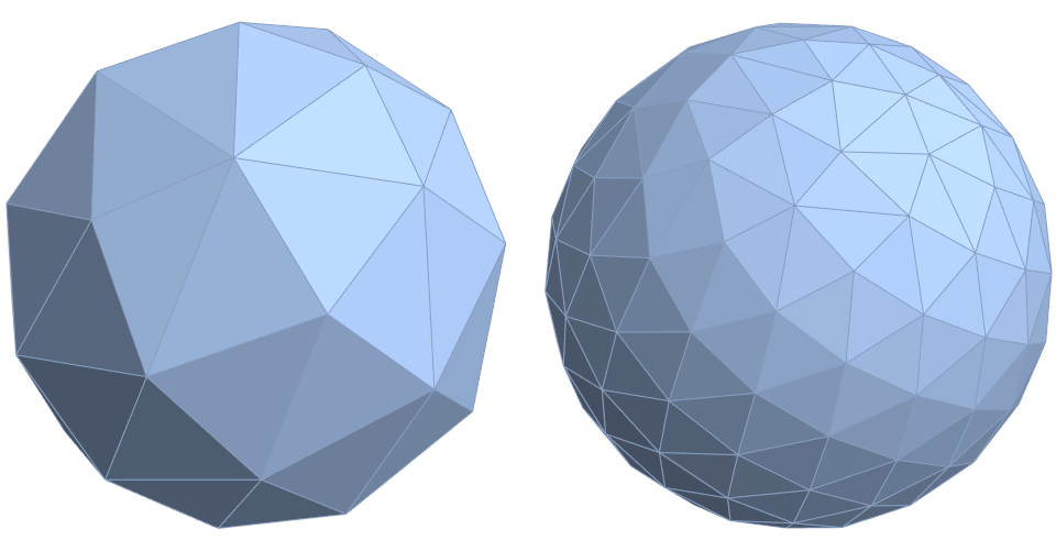
Also, the truncated icosahedron, which is the shape of a $C_{60}$ buckminster fullerene only corresponds to $d^{\ast }=3.125$.

Thus for $N>100$, lattices based on Eqn 3 are better than any geodesic polyhedra.

As per the first reference,  some of the state-of-the-art methods which are typically complex and require recursive and/or dynamic programming are as follows  (the higher the better).

$$\begin{array}{|lr|}\hline & d^{\ast }\\ \text{Coulomb}& 3.37\\ \text{Log Energy}& 3.37\\ \text{Lattice 3}& 3.34\\ \text{Zonal Equal Area}& 3.32\\ \text{Lattice 2}& 3.28\\ \text{Max Determinant}& 3.19\\ \text{Lattice 1}& 3.09\\ \hline\end{array}$$

Section 1 Summary

Lattice 3 (as defined in equation 4) produces a significantly tighter packing than the canonical Fibonacci lattice. That is,

$$t_0=(0,0);t_i=(\frac{i+\frac{7}{2}}{N+6},\frac{i}{\varphi });t_{N-1}=(0,1);\text{for }1\le i\le N-2$$

Section 2. Optimising the Convex hull (Delaunay mesh)

Although the previous section optimized for $d_N^{\ast }$, unfortunately these modifications actually make other measures worse, such as the volume of the convex hull (Delaunay mesh). This section shows how to evenly distribute points on a sphere in a manner that optimizes (maximizes)  a more global measure such as the volume of the convex hull.

Let us define $C_N$ as the convex hull of the $N$ points,

$${ϵ}_N=N(\frac{4\pi }{3}–\text{Vol}(C_N))$$

where the normalization factor of $N$ is included, because the absolute discrepancy decreases at a rate $1/N$.

The behavior of ${ϵ}_N$ for varying $N$ can be seen in Figure 3 (blue).

The key to improving the volume discrepancy is to note that although the use of $\varphi$, the golden ratio intuitively makes sense as $N\to \mathrm{\infty }$, it does not necessarily follow that it is the best value for finite $N$. In science terminology, we could say that need to consider finite-term correction effects.

Thus, let us generalize equation 1 as follows:

$$\begin{array}{}\text{(4)}& t_i=(\frac{i+1/2}{N},\frac{i}{g(N)})\text{for }0\le i\le N-1\end{array}$$

where we define $g(n)$ as follows:

$$\begin{array}{}\text{(5)}& g(n)=\{\begin{array}{ll}3-\varphi ,& \text{if }k\text{ is even}\\ \varphi ,& \text{if }k\text{ is odd}\end{array}\end{array}$$

where,

$$k=\lfloor {\text{log}}_{\varphi }(\frac{n}{1.5})\rfloor =\lfloor \frac{\ln (n/1.5)}{\ln \varphi }\rfloor$$

where $\lfloor x\rfloor$ is the floor function.

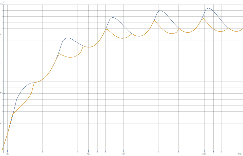
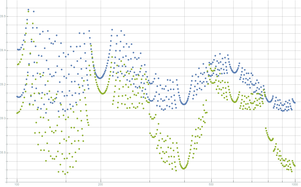
Figure 3 shows that this substantially improves the volume discrepancy for half the values of $N$.

The underlying reason why this works is based on the less well known fact that all numbers $x$ that satisfy the special Mobieus transformation are equivalent to $\varphi$ in terms of irrationality.

$$x=\frac{a\varphi +b}{c\varphi +d},\text{for all integers}a,b,c,d\text{such that }|ad-bc|=1$$

And thus the connection why $\varphi$ and $3-\varphi$ work together so well , is that

$$\frac{1}{\varphi }=\frac{\varphi +1}{2\varphi +1},\frac{1}{3-\varphi }=\frac{2\varphi +1}{1\varphi +1}$$

For the remaining half, we first define an auxiliary sequence $A_N$ that is variant of the Fibonacci sequence

$$A_1=1,A_2=4;A_{n+2}=A_{n+1}+A_n\text{for }n=1,2,3,\dots$$

That is,

$$A_N=1,4,5,9,14,23,37,60,97,157,254,411,\dots$$

The convergents of this sequence all have elegant continued fractions, and in the limit converge to $\varphi$. For example,

$$t_5/t_4=1+\frac{1}{1+\frac{1}{1+\frac{1}{1+\frac{1}{4}}}}$$.

We now fully generalize $g(n)$ as follows:

$$\begin{array}{}\text{(6)}& g(N)=\{\begin{array}{ll}3-\varphi ,& \text{if }k\text{ is even}\\ A_{j+1}/A_j,& \text{if }k\text{ is odd, where }j=(k+7)/2\end{array}\end{array}$$

The following table is a summary of the value of $g(N)$ for various $N$.

$$\begin{array}{|cccccccccc|}\hline N& 4-6& 7-10& 11-16& 17-26& 27-43& 44-70& 71-114& 115-184& 185-300\\ g(n)& 3-\varphi & \frac{23}{14}& 3-\varphi & \frac{37}{23}& 3-\varphi & \frac{60}{37}& 3-\varphi & \frac{97}{60}& 3-\varphi \\ \hline\end{array}$$

Figure 3 shows that, in relation to convex hull volume, this new distribution is better than the canonical lattice for all values of $n$.

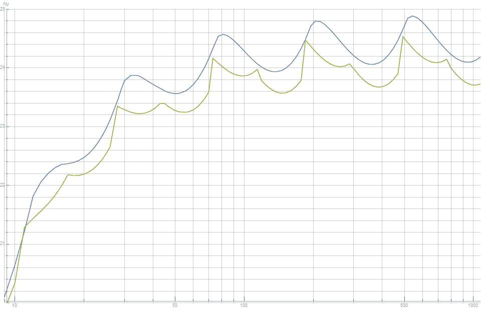
Figure 3. The discrepancy between the volume of the convex hull of points and the volume of a unit sphere. Note that smaller is better. This shows that the newly proposed method (green) produces consistently better distribution than the canonical Fibonacci lattice (blue).

Of interest, this distribution also slightly but consistently reduces the discrepancy between the surface area of the convex hull and the surface area of the unit sphere. This is shown in figure 5.

Section 2 Summary

The lattice as per equation 6, is a modification of the canonical Fibonacci lattice that produces a significantly better point distribution as measured by the volume and surface area of the convex hull (Delaunay Mesh).

Key References

• A Comparison of poopular point confugrations on S^2“:
• http://web.archive.org/web/20120421191837/
• http://www.cgafaq.info/wiki/Evenly_distributed_points_on_sphere
• https://perswww.kuleuven.be/~u0017946/publications/Papers97/art97a-Saff-Kuijlaars-MI/Saff-Kuijlaars-MathIntel97.pdf
• https://projecteuclid.org/download/pdf_1/euclid.em/1067634731
• https://maths-people.anu.edu.au/~leopardi/Leopardi-Sphere-PhD-Thesis.pdf
• https://www.irit.fr/~David.Vanderhaeghe/M2IGAI-CO/2016-g1/docs/spherical_fibonacci_mapping.pdf
• https://arxiv.org/pdf/1407.8282.pdf
• https://maths-people.anu.edu.au/~leopardi/Macquarie-sphere-talk.pdf

***

My name is Dr Martin Roberts, and I’m a freelance Principal Data Science consultant, who loves working at the intersection of maths and computing.

“I transform and modernize organizations through innovative data strategies solutions.”

You can contact me through any of these channels.

LinkedIn: https://www.linkedin.com/in/martinroberts/

Twitter: @TechSparx  https://twitter.com/TechSparx

email: Martin (at) RobertsAnalytics (dot) com

More details about me can be found here.

 

 

Other Posts you might like:

• Uniform Random sampling on an $n$-sphere an in an $n$-ball
• A new method to construct isotropic blue noise point sets with uniform projections
• Maximal Posison disc sampling: an improved version of Bridson’s algorithm.