I describe a how a small but critical modification to correlated multi-jittered sampling can significantly improve its blue noise spectral characteristics whilst maintaining its uniform projections. This is an exact and direct grid-based construction method that guarantees a minimum neighbor point separation of at least $0.707/n$ and has an average point separation of $0.965/n$.
The minimum nearest neighbor distance is guaranteed to exceed $0.707/n$ and the average distance is $0.965/n$. Their blue noise sample point distributions are isotropic and their 1-D projections are exactly uniformly distributed. Futhermore each set can be directly and exactly constructed through just two permutations of the $n$-dimensional vector $\{1,2,3,…,n\}$. This therefore, presents a new way of directly constructing tileable isotropic blue noise without the need for iterative methods such as best candidate or simulated annealing
First published: 1st April, 2020
Last updated: 17 April, 2020
0. Introduction.
In many applications in math, science and computing, generating samples of points from a blue noise distribution is particularly important.
In this post, we show how to construct a set of points, for arbitrary $N$, such that:
-
- the points are evenly distributed across the unit square
- it has a guaranteed min distance between neighboring points
- there is a large average distance between neighboring points
- it has a blue power spectrum
- its point distribution is very close to isotropic
- it has exactly uniform 1D projections
Furthermore, the method is an exact and direct grid-based construction method, which means that unlike many contemporary methods, this new method does not require randomization, greedy selection, iterative sampling, or relaxation methods to progressively sample, identify or adjust the position of the points into optimal locations.
Before proceeding, it is very important to note that unlike almost all my other blog posts relating to quasirandom blue noise sequences, this post describes the construction of a set of $N$ points that exhibit blue noise characteristics. A set is a collection of items that has no intrinsic ordering. The construction and the main desirable attributes of such as set only makes sense when all points in the set are considered in their entirety. This distinct lack of ordering means that this construction method is in the same category as solving the $N$-rooks/queens problem, orthogonal arrays, digital $t-$nets, Latin squares and valid sudoku puzzles.
Contrast this to a sequence of points, which is an ordered collection of items. Many blue noise point distributions are constructed via a sequence that defines a specific ordering of geometric points in $d$-dimensions. Usually the underlying sequence is a low discrepancy sequence (eg see my post “A simple method to construct isotropic quasirandom blue noise point sequences“). However, other approaches include iterative greedy selection (eg “An improved version of Bridson’s algorithm for Poisson disc sampling“). Regardless of which approach is used, a sequence is constructed one point at a time; and for any $k<N$ there is meaningful value at looking at the configuration of the first $k$ points.
1. Canonical Configuration
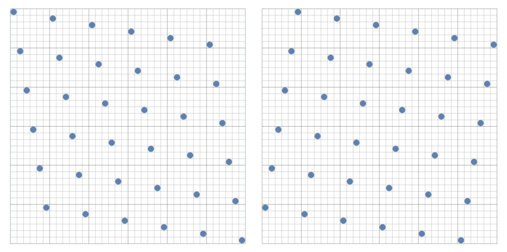
Two very common methods to distribute grid-based points that are very nearly optimally spaced apart, whilst ensuring that the projections are exactly uniformly distributed are shown in figure 2. Note for both variations, there is exactly one point in every row, every column, and every block. These row and column constraints mean the projections are uniformly distributed, and the block-constraint drives the equal-spacing between neighboring points. However, due to the high degree of regularity, the fourier transform exhibits extremely strong peaks and is definitely not isotropic. Nor does it exhibit the classic blue noise power spectrum.
The version on the left is the most popular layout, whilst the version on the right is often called the ‘rotated grid’. In most contexts (including this blog post) it’s standard to consider ‘wrapped’ edges, that is, the grid is topologically equivalent to a torus, which allows for tiling. For the first variant, if the grid is tiled, then the top-left point will be extremely close to the lower-right point. If the second variant is tiled, then the top-left region and the bottom-right region will form a undesirably large gap. Thus, although they both have subtly different strengths and weaknesses, for this post I will use the second variant.
(In another mini blog post, “An alternate canonical grid layout” I give details on an improved variant of the canonical layout.)
Note that for both versions, the average distance between neighboring points is consistently very large $\simeq 1/n$, and that the 1D projections are uniformly distributed. However, the obvious regularity means that they are not isotropic and exhibit fourier peaks. This often results in undesirable aliasing or degenerate effects.
2.Correlated Shuffling
A surprisingly easy way to make a point set very nearly isotropic, is to begin with a canonical grid and then shuffle the $n$ block-level rows and then shuffle the $n$ block-level columns.
Several examples of the shuffled canonical configurations are shown in figure 2.
This approach is described in the paper “Correlated Multijittered Sampling” by Kensler (though it is described quite differently), which in turn was based on the paper “Multi-Jittered Sampling” (1994) by Chui, Shirley and Wang. (Preumsably, it was termed ‘correlated shuffling’ because each time a colum-block is shuffled, all points within that column-blocks are displaced in the same way.)
This simple correlated shuffle produces a set of points that are more evenly distributed than either jittered uniform grid sampling or an $N$-rooks uncorrelated shuffling configuration. Unfortunately, as Kensler points out, a small but significant fraction of generated patterns contain at least one pair of points that are diagonally quite close to each other (see especially top-left and lower-left examples in figure 2).
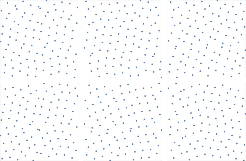
The points are generally well-spaced, the point distribution is virtually isotropic, and the 1D projections are still uniformly distributed. The average neighboring distance is $0.906/n$. However, in some instances the minimum neighboring distance can be as quadratically small as $1.414/n^2$ (eg see especially the top-left and bottom-left examples).
3. An improved Sampling method
Ideally, we would like to shuffle the canonical grid well enough to ensure that the regularity disappears, but gently enough that neighboring points stay well separated. That is, perturbations that are large enough for the fourier transform to have no peaks; but small enough to maintain the classic blue noise power spectrum.
We now describe a simple method that achieves an excellent balance between these two competing criteria.
Suppose we consider the finite sequence $\{1,2,3,4,5,6\}$.
Now consider a permutation of this sequence
$$\sigma = \{ \sigma_1, \sigma_2, \sigma_3, \sigma_4, \sigma_5, \sigma_6\}$$
We then define the first-order difference sequence $\delta$, as
$$\delta \equiv \{\sigma_2 {-} \sigma_1, \sigma_3 {-} \sigma_2, \sigma_4 {-} \sigma_3, \sigma_5 {-} \sigma_4, \sigma_6 {-} \sigma_5, \sigma_1 {-} \sigma_6\}.$$
Note that the last term is wrapped because we wish to consider the sequence as a cyclic permutation.
For example if $\sigma = \{3,2,6,1,5,4\}$, then $\delta = \{ -1,+4,-5,+4,-1,-1 \}$.
It should be clear that no matter how we permute the original sequence, each term in the difference sequence will be an integer in the range $[-5,5]$, and there could be repeated values.
Let’s now consider the permutation $\sigma = \{6,4,5,2,1,3\}$ as it has a particularly interesting property.
In this case, $\delta = \{-2,+1,-3,-1,+2,+3\}$. We specifically note that all these terms fall in a much smaller interval range $[-3,3]$, and furthermore all the terms are distinct.
That’s pretty cool. Actually, this is very cool and is more formally articulated as:
For $n=2k$, a permutation $\sigma_n$ is said to be balanced if all elements of the difference vector $\bf{\delta}$ are unique and lie in the range $[-k,+k]$.
That is, $\sigma_n$ is a balanced permutation if, and only if, $\delta$ is a permutation of $\{{-}k,{-}k{+}1,…,-2,-1,+1,+2,…k{-}1,+k\}$.
Therefore, our first permutation example $\{3,2,6,1,5,4\}$ is not balanced, but the second example $\{6,4,5,2,1,3\}$ is balanced.
The following tables lists some more examples of balanced permutations for various $n$.
\begin{array}{|l|ll|} \hline
n & \sigma_1 & \delta \\ \hline
4 & \{1, 2, 4, 3\} & \{+1, +2, -1, -2\} \\
4 & \{1, 3, 4, 2\} & \{+2, +1, -2, -1\} \\ \hline
6 & \{6, 4, 5, 2, 1, 3\} & \{-2, +1, -3, -1, +2, -3\} \\
6 & \{2, 5, 4, 6, 3, 1\}& \{+3,-1,+2,-3,-2,1\} \\ \hline
8 & \{1, 2,6, 8, 5, 4, 7 ,3\} & \{+1, +4, +2, -3, -1, +3, -4, -2 \} \\
8 & \{1, 4, 8, 6, 7, 3, 5, 2\} & \{+1, -4, +2, -3, -1, +3, +4, -2 \} \\ \hline
16 & \{ 16,11,5,1,2,8,15,7,9,14,13,10,3,6,4,12 \} & \{ -5,-6,-4,+1,+6,+7,+2,+5,-1,-3,-7,3,-2,8,4\} \\
16 & \{ 1,9,15,12,4,11,16,14,7,3,5,6,10,13,8,2 \} & \{ +8,+6,-3,-8,+7,+5,-2,-7,-4,+2,+1,+4,+3,-5,-6,-1\} \\ \hline
20 & \{1, 6, 2, 10, 20, 12, 5, 4, 7, 14, 16, 17, 8, 3, 9, 18, 15, 19, 13, 11\}, \\
& \{1, 9, 15, 7, 10, 3, 5, 6, 13, 4, 14, 19, 18, 16, 20, 17, 12, 8, 2, 11\} \\ \hline
\end{array}
We can now state our major result:
If $\bf{\sigma_1, \sigma_2}$ are balanced permutations, then permuting the block-columns of the canonical grid via $\bf{\sigma_1}$ and then the block-rows via $\bf{\sigma_2}$, will result in an isotropic point distribution whose neighboring points are guaranteed to be at least $\bf{1/(\sqrt{2}n)}$ apart, and which has exactly uniformly distributed projections.
Thus, we may permute the canonical grid in a fully deterministic manner using any two (preferably different) balanced permutations. For example, in figure 4, beginning with canonical grid (second variant), the row blocks have been permuted with $\sigma_1 = \{1,5,8,7,4,6,2,3\}$ and the column-blocks with the permutation $\sigma_2 = \{1,3,2,6,4,7,8,5\}$.
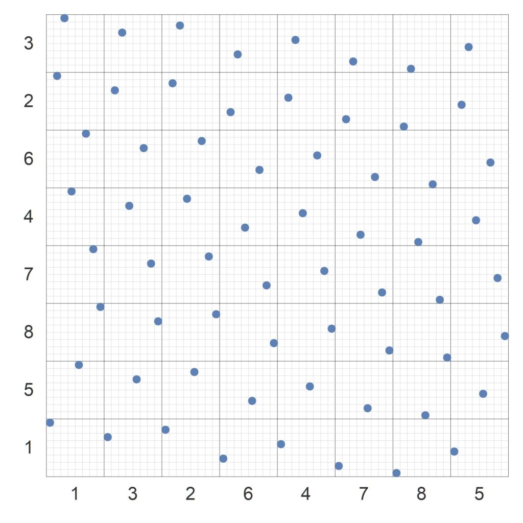
Beginning with the canonical grid, the row-blocks have been shuffled using the balanced permuation $\{1,5,8,7,4,6,2,3\}$ and then the column-blocks have been shuffled using the balanced permutation $\{1,3,2,6,4,7,8,5\}$. The 1-D projections are therefore still exactly uniform, the fourier transform is virtually isotropic, and the minimum nearest neighbor distance is now always at least $0.707/n$ and the average distance is $0.965/n$.
And since both permutations are cyclic, the final point set is tileable.
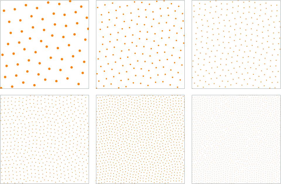
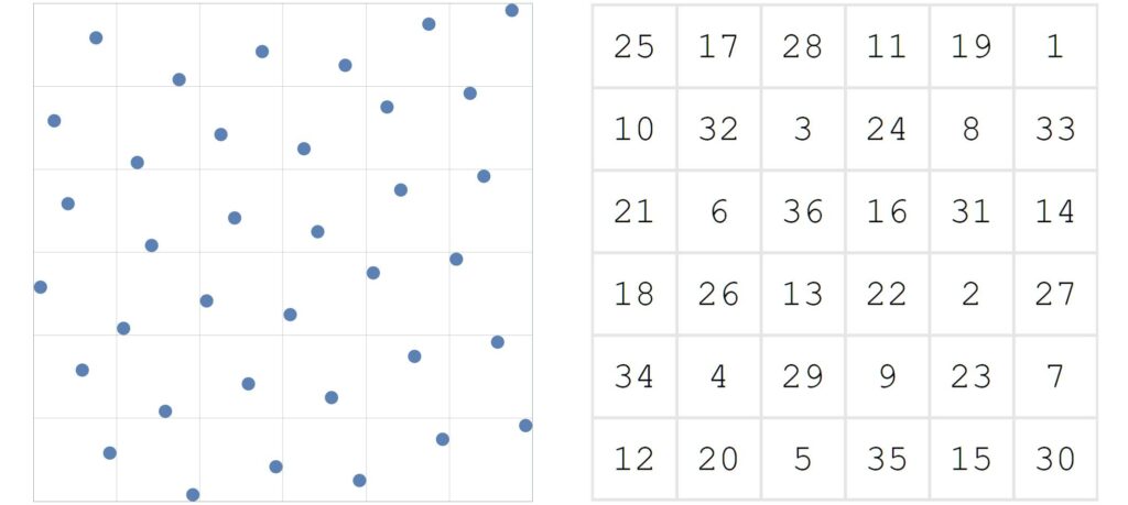
Figure 5 shows several more examples of $n^2$ point sets $(n=10)$ created through this technique. The average separation between neighboring points is $0.965/n$. And in all examples, the minimum separation exceeds $1/(\sqrt{2}n)$. Also, recall that figure 1 shows examples of balanced shuffles for $n=8,12,16,24,32, 40$.
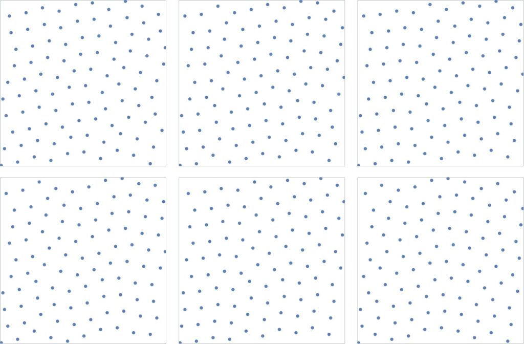
Each set of $n^2$ points can be described and constructed through just two special permutations of the n-vector $\{1,2,3,…,n\}$.
4. Constructing balanced permutations
The following permutations are excellent default values for various $n$.
\begin{array} \hline
n & \sigma \\ \hline
6 & \{ 1,3,2,5,6,4 \} \\
& \{ 1,2,5,4,6,3 \} \\ \hline
8 & \{ 1,4,2,3,7,6,8,5 \} \\
& \{ 1,3,2,6,4,7,8,5 \} \\ \hline
10 & \{ 1,4,9,10,8,5,7,3,2,6 \} \\
& \{ 1,5,10,7,9,8,4,2,3,6 \} \\ \hline
12 & \{ 1,6,9,4,3,5,2,8,12,10,11,7 \} \\
& \{ 1,6,5,2,4,10,11,9,12,8,3,7 \} \\ \hline
16 & \{ 1, 7, 5, 6, 14, 8, 12, 15, 10, 3, 2, 4, 11, 16, 13, 9 \} \\
& \{ 1, 8, 6, 10, 3, 4, 12, 15, 14, 16, 11, 5, 2, 7, 13, 9 \} \\ \hline
20 & \{ 1,9,19,13,6,2,8,3,10,7,12,4,5,14,18,16,15,17,20,11 \} \\
& \{ 1,10,5,8,4,6,12,17,14,18,16,7,15,9,2,3,13,20,19,11 \} \\ \hline
24 & \{ 1,2,5,7,19,8,3,11,9,6,16,10,17,21,14,4,15,24,20,12,18,23,22,13 \} \\
& \{ 1,12,7,5,10,20,9,15,18,14,23,22,19,21,11,3,4,16,24,17,8,2,6,13 \} \\ \hline
32 & \{ 1,6,22,11,12,7,16,4,8,2,10,24,21,31,18,14,29,15,28,19,26,25,27,30,23,13,5,3,9,20,32,17 \} \\
& \{1,11,10,14,3,19,15,21,30,28,25,32,26,12,24,27,22,9,2,7,8,16,31,23,13,4,6,20,5,18,29,17 \} \\ \hline
\end{array}
However, if you wish to calculate arbitrary balanced permuations, the following python code randomly generates a balanced permutation of length $n$.
import random as rs
def getBalanced(n):
  balanced = []
  allowedItems = {1}
  allowedSteps = []
  for i in range(1, int(n/2)+1):
    allowedItems.add(i)
    allowedItems.add(i+int(n/2)
    allowedSteps.append(i)
    allowedSteps.append(-i)
    pass
  balanced.append(1)
  allowedItems.remove(1)
  rs.shuffle(allowedSteps)
  def getNextElement(balanced, allowedItems, allowedSteps):
    if allowedItems == set() and (balanced[0] - balanced[-1]) in allowedSteps:
      return balanced
    elif allowedItems == set():
      return []
    else:
      for step in allowedSteps:
        if (step + balanced[-1]) in allowedItems:
          balancedTemp = balanced.copy()
          balancedTemp.append(step + balanced[-1])
          allowedItemsTemp = allowedItems.copy()
          allowedItemsTemp.remove(step + balanced[-1])
          allowedStepsTemp = allowedSteps.copy()
          allowedStepsTemp.remove(step)
          theList = getNextElement(balancedTemp, allowedItemsTemp, allowedStepsTemp)
          if theList != []:
            return theList
            break
          pass
        pass
      return []

  balanced = getNextElement(balanced, allowedItems, allowedSteps)
  return balanced
# method to verify that a sequence is balanced
def differences(arr):
    seq = arr
    seq.append(arr[0])
    d = [i-j for i,j in zip(seq[1:], seq[:-1])]
    d.sort()
    return d
# Prints a randomly generated balanced sequence of length 16.
print(getBalanced(16))
Update 2nd April 2020. Tommy Ettinger has provided corresponding Java code which is around 20x faster than this python code. As an indication, it generates balanced permutations of length $n=16$ in about one millisecond, and balanced permutations of length $n=56$ in about one second.
Update 17th April 2020. Max Tarpini has provided corresponding C/C++ code which is around 30% faster again than the Java version.
Here is a pre-computed list of Balanced Permutations for various $n$. It is contains the fully enumerated list for $n \leq 12$ , and a few hundred randomly generating balanced sequences for $n=16,24,32,40,48,56,64$.
Note that for any balanced permuation $\sigma = \{ \sigma_1, \sigma_2, \sigma_3,\ldots, \sigma_n \}$,
- Any cyclic permutation of $\sigma$ is also a balanced permutation (rotations).
- $\{\sigma_n, \ldots, \sigma_3, \sigma_2, \sigma_1\}$ is also a balanced permutation. (reflections)
- $ \{ n+1-\sigma_1, n+1-\sigma_2, n+1-\sigma_3,\ldots, n+1-\sigma_n \}$ is also a balanced permutation (inversions).
Enumerating permutations
Accounting for rotations, reversals and inversions:
- For $n=6$, there are 24 distinct balanced permutations, which correspond to $24^2= 576$ different blue-noise point sets.
- For $n=8$, there are 92 distinct balanced permutations, which correspond to over 9,000 different blue-noise point sets.
- For $n=10$, there are 1,060 distinct balanced permutations, which correspond to over one million different different blue-noise point sets.
- For $n=12$, there are 8,568 distinct balanced permutations, which correspond to over 73 million different blue-noise point sets.
- For $n=14$, there are over 170,000 distinct balanced permutations, which correspond to over 280 billion different blue-noise point sets.
- For $n=16$, there are over 3.3 million distinct balanced permutations, which correspond to over 10 trillion different blue-noise point sets.
Fourier Analysis
We compare the fourier transform and power spectra of a balanced shuffle point set with that of a simple correlated shuffle point set.
For a more detailed comparison of the various contemporary point distributions and their fourier spectra, see “Progressive Multi-jittered Sampling“.
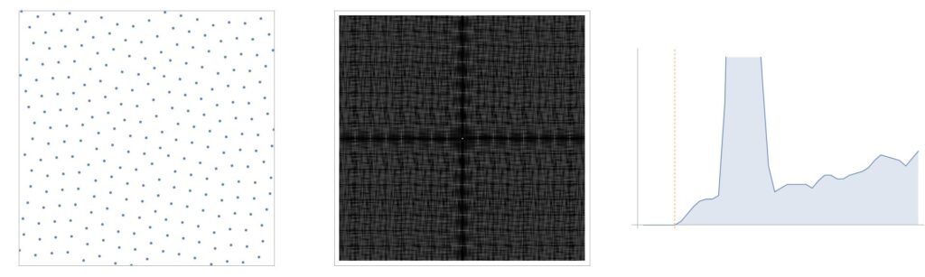
The point distribution, fourier transform and power spectrum for a balanced shuffle $(n=16)$. The point distribution is isotropic as seen by the fact that the fourier spectrum is relatively uniform and clearly has no peaks. The large minimum and average distance between neighboring points results in the complete absence of low frequencies below the orange dotted line, as well as the central circle in the fourier spectrum. The large horizontal and vertical band is because for any given point, there are never any other points in the same row or column.
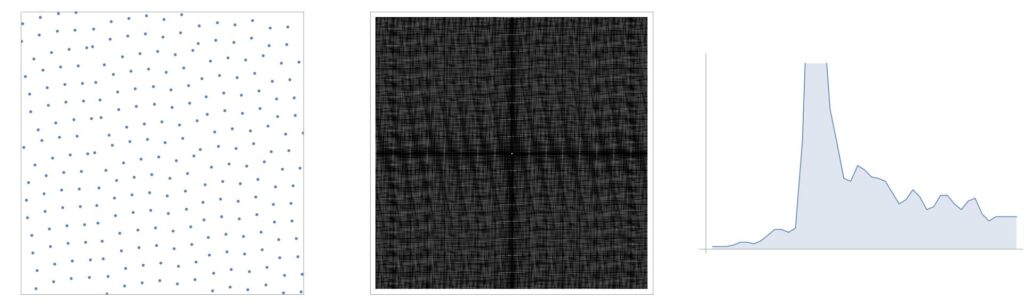
The point distribution, fourier transform and power spectrum for a simple correlated shuffle $(n=16)$. Note that the Fourier transform is not as smooth. Also the existence of a small number of pairs of points very close to each other results in a power spectrum that is small but not zero for the lowest frequencies. Also note that the much smaller central circle as well as the vertical & horizontal black bars in the fourier spectrum are much less apaprent for the correlated shuffle.
The fourier transform’s lesser known cousin is the pair correlation function. This function focuses on the relative position of neighboring points. That is, for each point $\bf{p_i}$, let $\bf{q_{ij} }$ be the $j$-th nearest neighbor. Then define $\bf{r_{ij}} \equiv \bf{q_{ij}} – \bf{p_{ij}}$.
By graphing the $\bf{r_{ij}}$ for each of the $N$ points for $1 \leq j \leq k$, we can clearly visualize see the relative directions and distances of the $kn$ closest neighbors. Figure 7 shows the value for $k=1$.
Interestingly, this observed 8-fold pattern could be interpreted that balanced permuations produce isotropic point distributions under the Manhattan (‘taxi cab’) $\ell_1$-norm rather then the usual Euclidean $\ell_2$-norm. For further explorations in the direction see “Anistropic Blue Noise sampling” by Wei.
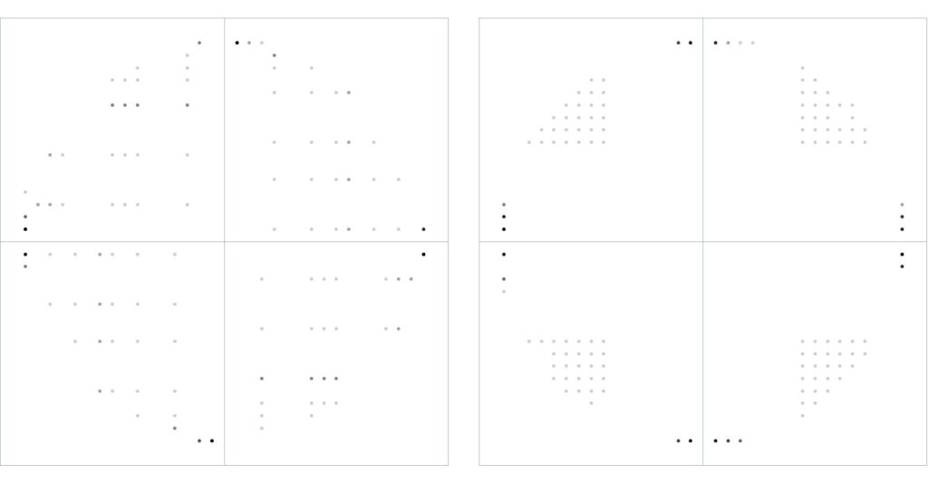
Correlated shuffling (left) is fairly isotropic, but also only a small minimum neighboring distance. In contrast, balanced shuffling shows an clear pattern 8-fold pattern, as well as a very clear minimum neighbor distance.
Progressive Sampling
Although the $N=n^2$ points do not have an intrinsic underling order, it is possible to order them in a way such that the region is progressively and evenly filled.
The key to this ordering is through the use of any $n \times n$ ordered dither matrix, $\mathcal{D}$. Since each block contains exactly one point, then there is an obvious 1:1 mapping between the $n^2$ points points in the shuffled grid and the $n^2$ cells in the dither matrix.
For the example shown in figure 8, the first point of the progressive sequence would be the top left-most point. Again, note that there is nothing special about this particular dither matrix. Any ordered dither matrix is sufficient, as all dither matrices are designed to admit a progressive sequence.
Thus, the points can be trivially ordered and therefore we can create a progressive sequence of $n^2$ low discrepancy points (the progressive degree of isotropy and uniformity of its projections is based on the quality of the dither matrix itself).
Most high quality dither matrices are constructed through the iterative void-and-cluster method. However, for this context a fairly good dither matrix can be directly constructed using a simple linear congruential generator. For example, consider the sequence (often called the lagged Fibonacci sequence),
$$F_n = \{1,1,2,3,4,5,7,9,12,16,21,28,37,49,65,86,114,151,200 \} \quad \textrm{where} \; F_{k+3} =F_{k+2} + F_k$$
Then from this we define $g$ as the positive real root of the characteristic equation $x^3 = x^2+1$. This is equivalent to the following definition.
$$ g =\lim_{n\to \infty} \;\;\frac{F_{n+1}}{F_n} .$$
Then for any real number $s$, define the auxiliary square matrix $B$ such that
$$ B_{ij} = (s + i/g+ j/g^2) \;\; \%1 $$
where the $(\cdot) \; \%1$ notation denotes the fractional operator.
Then define $\mathcal{D_{ij}}$ as the rank of $\mathcal{B_{ij}}$ in $\mathcal{B}$. (That is, simply select the cells of $\mathcal{B}$ in ascending order.)
Note that a very similar generator based on the sequence $F_{k+3} =F_{k+1} + F_k$ and its characteristic equation $x^3=x+1$ is discussed in detail in my blog post, “The unreasonable effectiveness of quasirandom sequences“.
Shuffling the canonical grid with a balanced permutation (left) still results in exactly one point per block. This allows a trivial 1:1 mapping between the $n^2$ points, and the $n^2$ cells in a ordered dither matrix, $\mathcal{D}$ (right). Thus, the first point in the sequence would be the top-right point.
Point distributions for arbitrary $N$
So far we have only discussed methods for constructing a set of $N$ evenly-distributed points if $N$ is a perfect square, that is $N=n^2$, for some $n$.
We present an improved version of an approach first discussed in “Correlated Multi-jittered Sampling” to allow point distributions for any $N$.
Consider figure 4, where $n=8$ there are $n^2=64$ points distributed among 64 rows and 64 columns.
From this it is surprisingly simple to create a distribution that has, say only $N=53$ points. We note that as the balanced shuffling always results in exactly uniform projections, there will be eactly one point in the very top row and exactly one point in the far column. Thus, we simply start slicing off the top row, and then slice off the the far column, and then the next top row, and then the next far column, until we only have $N=53$ points left.
Thus, after deleting the top 6 rows and 5 rightmost columns, we will have 53 points. (Unfortunately, the small cost of allowing arbitrary $N$ is that the resulting point distribution will no longer be cyclic).
The result of this protocol will be a always be a shape that is a square or extremely close to a square. In our case, 58 rows by 59 columns. Now we simply scale the horizontal axis by a factor of (64/58) and the vertical axis by a factor of 64/59, and we are done. This method ensures that the 1-D projections are still uniform. The fact that the sliced shape is always almost-square ensures that 2D-distortions are minimized, and that both the distances and relative directions between neighboring points (and thus isotropy) is essentially preserved.
Tiling
Constructing permutations for $n<45$ is relatively simple and so blue-noise point distributions for $N<2000$ can be easily constructed. An easy way to construct a point set for much larger values of $N$ is to simply tile smaller sets together. The standard approach to tiling is to tile identical copies of a base image. However, this approach often results in either undesirable edge alisasing artefacts and/or visible large-scale regularities.
Our new point-set construction method transforms a geometric problem into an algebraic problem. This means that if two permutations are algebraically similar, then they will produce similar geometric point distributions. This in turn, means that we can easily tile similar, but different, base tiles together with minimal aliasing!
We can achieve this by first forming a set of balanced permutations that are all similar to one and another (such as below). We then generate multiple point sets — each based on a randomly selected pair of permutations from this basis set. When we tile these similar but different point sets together, there will be minimal edge-aliasing or signs of large-scale regularity. This infinte quasiperiodic construction using a finite number of unit tiles, is similar in many ways, to Wang tiles and Penrose Tilings.
Below is the result of 54 different base units ( $n=10$) arranged in a $9\times 6$ layout using this method and the following basis set:
$$ \{1,2,7,10,5,9,6,8,4,3\}, \quad \{1,2,7,10,6,8,5,9,4,3\},\quad \{1,2,7,10,8,4,3,5,9,6\}, \quad \{1,2,7,10,9,6,4,8,3,5\} $$

In this case, 54 smaller sets, each with $10^2$ points have been tiled together. Each unit tile was generated using pairs of similar but different permutations. Therefore, there is no periodicity and almost no edge-based artefacts.
Jittering
Although there are many advantages to having exactly uniform projections and grid-based sampling, if you don’t want them to be exact, you can simply add a sub-cell (sub-pixel) jitter to each coordinate of each point. The magnitude of the jitter simply needs to be less than $1/n^2$ in either axis direction.
Convergence rates in Monte Carlo methods
When point sets generated with balanced shuffling are used in Quasi-Monte Carlo methods, the convergence rate is excellent, and identical to when point sets generated with correlated shuffling (a.k.a. simple or progressive multijittered sampling ‘pmj’) are used.
For example, when integrating functions with discontinuous non-differentiable hard edges (such as $x^2+y^2 \leq r^2$, the convergence rate is ~$n^{-0.75}$. In contrast, when integrating functions with smooth differentiable edges (such as Guassians) the convergence rate is even better at $n^{-1}$ (not shown). See “Progressive Multijittered Sampling” by Christensen et al, for more details on this.
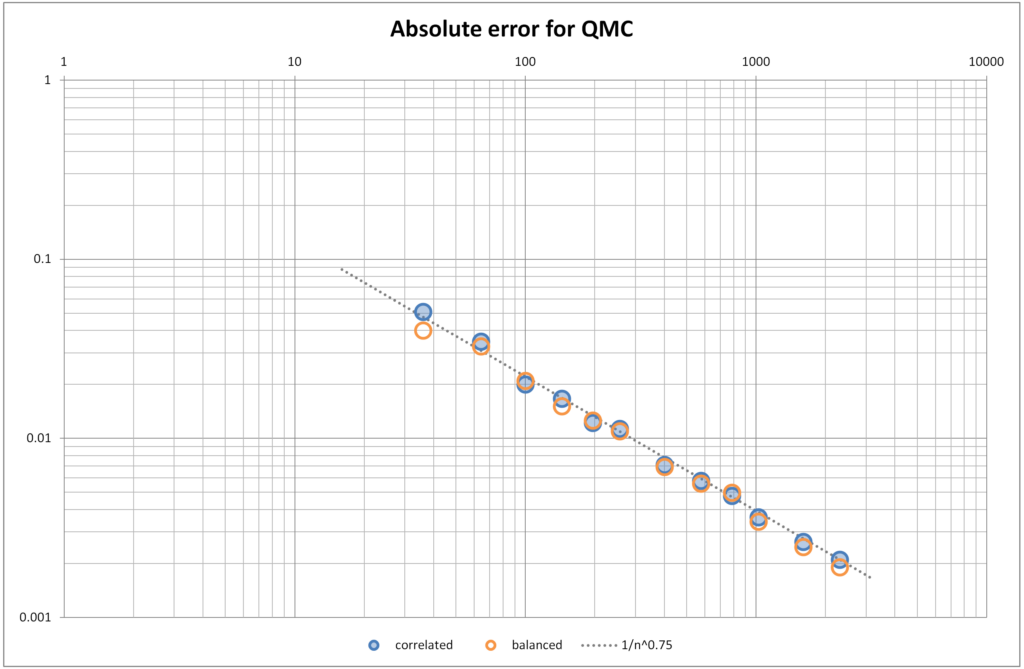
Convergence of QMC using correlated and balanced shuffling for a disk function. Note that both converge at a rate of $1/n^{0.75}$.
Higher dimensions
It is quite plausible, that if one can determine the generalization of a canonical layout in higher dimensions (preferably it would be a rotated $n$-cube, but alternatively it might be similar to th ethe canonical layouts described in table 2 of “Orthogonal Array Sampling for Monte Carlo Rendering”) then this method could be used to produce higher-dimensional blue noise distributions that have also uniform projections. Hopefully future blog posts will explore this avenue further.
Conclusion
We have described a simple method for an exact and direct construction of tileable isotropic blue noise grid-based sample d point sets that that have:
-
- a guaranteed minimum neighboring distance of $1/(\sqrt{2}n)$
- an average separation of $0.965/n$
- projections that are uniformly distributed.
And this is all achieved simply by using two balanced permutations: one to permute the block-rows of a canonical layout, and another to then permute the block-columns. Where a permutation $\sigma$ of length $n=2k$ is balanced when all the elements of its difference vector are unique and lie in the range $[-k,+k]$. That is, $\sigma_n$ is a balanced permutation if $\delta$ is a permutation of $\{{-}k,{-}k{+}1,…,-2,-1,+1,+2,…k{-}1,k\}$.
Intuitively, the condition that the differences $|\delta_i| \leq k$ forces the guaranteed minimum separation and drives the consistently high average separation between neighboring points. Whereas the condition that the $\delta_i$ are unique, ensures that the point distribution is isotropic.
We have briefly outlined a method how, through the use of a dither matrix, that these point-sets can transformed into an ordered progressive finite sequence.
Furthermore, although this method mainly and naturally applies to points sets of cardinality $N=n^2$, we have also outlined a method to produce balanced point-sets of arbitrary cardinality.
The fact that each point set is fully and exactly described via two permutations, means that we have transformed a geometric problem into an algebraic problem. Thus, a similar permutation will create a geometrically similar point set. One application of this elegant principle is that we can tile different point sets together in a manner that exhibits almost no undesirable edge aliasing or large-sale regularity. This method can actually be used like Wang tiles to create infinite non-periodic tilings using only a set of finite number of tiles.
Another advantage of these permutation-defining configurations, is that they are like a seed in a random generator. That is, we can randomly select two permutations to create a point distribution, and then allow third-parties to exactly replicate the results by simply referencing the two specific permutations we used.
Finally, we have briefly shown that the convergence rate for Quasi-Monte Carlo methods is excellent and identical to that of correlated shuffling (ie progressive multi-jittered sampling).
It is hoped that due to the simplicity of this method as well as many of its elegant properties, that it could be used in a wide variety of mathematical, scientific and computing applications where blue noise point sets are required.
***
My name is Dr Martin Roberts, and I’m a freelance Principal Data Science consultant, who loves working at the intersection of maths and computing.
“I transform and modernize organizations through innovative data strategies solutions.”You can contact me through any of these channels.
LinkedIn: https://www.linkedin.com/in/martinroberts/
Twitter: @TechSparx https://twitter.com/TechSparx
email: Martin (at) RobertsAnalytics (dot) com
More details about me can be found here.