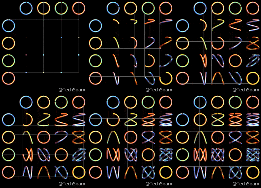
This post illustrates and explains the beautiful Lissajous Curves – trajectories of points whose coordinates follow sinusoidal movements. A simple but timeless classic curve that has numerous applications as well as artistic elegance.

Introduction

Lissajous curves are the family of curves described by the parametric equations:

\begin{array}{rl}
x(t) &= A \sin [a (t-\theta)] \nonumber \\
y(t) &= B \cos [b(t + \theta)] \nonumber \\
\end{array}

There is lots of information on the web about these these curves , including

In the most common renderings, the phase shift $\theta$ is set to zero, and $t$ is steadily increasing.

For various values of $a,b$ you get different patterns. For example,

If $a = b, \theta = 0$ then the curve is a circle
For $a \neq b, \theta = 0$, you get an ellipse.
For $a= b, \delta = \pi/2$, you get a parabola.
For $a = 3; b=1, \theta = 0$, you get a the well-known “Australian Broadcasting Commission”, logo.

Dynamic Phase

When you look closely you will notice that it is generally symmetrical, that is $a=1,b=3$ gives the same result as $a=3,b=1$, just rotated.

However, more astute readers will notice that it is not exactly symmetrical. For example $a=1;b=2$ appears quite different to $a=2,b=1$.

The reason for this is because in its current rendering the pair of equations is not exactly symmetrical. One uses $sin(\cdot)$ and the other used $\cos(\cdot))$. If you plot these on a normal graph you will notice that they are effectively the same shape but just shifted. That is, there is a hidden phase difference between these two equations.

To make this phase more explicit, we can keep the $t$ domain constant and vary the phase, \theta.

\begin{array}{rl}
x(t) &= A \sin [a (t-\theta)] \nonumber \\
y(t) &= B \cos [b (t + \theta)] \nonumber \\
\end{array}

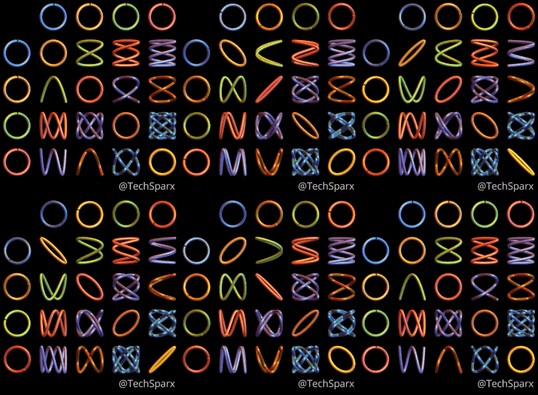
Note that top row and first column indicate the varying relative phase difference.

The consequence of this is the grid is now fully and symmetrical.

For example, you will see that $a=1, b=2$ is now just rotated version of $a=2, b=1$ as we would expect.

Roses

A family of curves related to the Lissajous curves are the roses.

\begin{array}{rl}
x(t) &= \cos (k t) \cos t \nonumber \\
y(t) &= \cos (k t) \sin t \nonumber \\
\end{array}

Here are two examples:

Rose (1,3)

Rose (2,3)

Enjoy!

My name is Martin Roberts. I have a PhD in theoretical physics. I love maths and computing. I’m open to new opportunities – consulting, contract or full-time – so let’s have a chat on how we can work together!

Come follow me on Twitter: @Techsparx!

My other contact details can be found here.

[mc4wp_form id=”1021″]

Introduction

Dynamic Phase

Roses

Other Posts you may like